Diffusion Models Miscellany (29): Discrete Coding with DDPM

生成扩散模型漫谈（二十九）：用DDPM来离散编码 苏剑林 · 2025-02-14 · Machine Learning generative model encoding DDPM diffusion discretization

A couple of days ago I stumbled across a new paper on arXiv, Compressed Image Generation with Denoising Diffusion Codebook Models, and I was genuinely amazed by the author's wild imagination — I couldn't resist sharing it with everyone.

As the title of this post suggests, the authors propose an idea called DDCM (Denoising Diffusion Codebook Models), which restricts DDPM's noise sampling to a finite set. This turns out to enable some remarkable effects, such as encoding samples into discrete ID sequences and reconstructing them back, much like VQVAE. Notably, all of this is done on top of a pretrained DDPM, with no additional training required.

Finite Set

Since DDCM only needs a pretrained DDPM model to perform sampling, we won't repeat the details of the DDPM model here. Readers who aren't yet familiar with DDPM can review parts (1), (2), and (3) of our Diffusion Models Miscellany series. more

As we know, DDPM's generative sampling starts from $\boldsymbol{x}_T\sim\mathcal{N}(\boldsymbol{0},\boldsymbol{I})$ and iterates to $\boldsymbol{x}_0$ via the following equation:

\begin{equation}\boldsymbol{x}_{t-1} = \boldsymbol{\mu}(\boldsymbol{x}_t) + \sigma_t \boldsymbol{\varepsilon}_t,\quad \boldsymbol{\varepsilon}_t\sim\mathcal{N}(\boldsymbol{0},\boldsymbol{I})\label{eq:ddpm-g}\end{equation}

For DDPM, each iteration step requires sampling a noise vector, and together with $\boldsymbol{x}_T$ itself being sampled noise, over $T$ iteration steps generating $\boldsymbol{x}_0$, a total of $T+1$ noise vectors are fed in. Assuming $\boldsymbol{x}_t\in\mathbb{R}^d$, DDPM's sampling process is essentially a mapping of the form $\mathbb{R}^{d\times (T+1)}\mapsto \mathbb{R}^d$.

DDCM's first flash of insight is to replace the noise sampling space with a finite set (a codebook):

\begin{equation}\boldsymbol{x}_{t-1} = \boldsymbol{\mu}(\boldsymbol{x}_t) + \sigma_t \boldsymbol{\varepsilon}_t,\quad \boldsymbol{\varepsilon}_t\sim\mathcal{C}_t\label{eq:ddcm-g}\end{equation}

as well as $\boldsymbol{x}_T\sim \mathcal{C}_{T+1}$, where $\mathcal{C}_t$ is a set of $K$ noise vectors pre-sampled from $\mathcal{N}(\boldsymbol{0},\boldsymbol{I})$. In other words, before sampling even begins, we draw $K$ vectors from $\mathcal{N}(\boldsymbol{0},\boldsymbol{I})$ and fix them; every subsequent sampling step then draws uniformly from these $K$ vectors. In this way, the generation process becomes a mapping of the form $\{1,2,\cdots,K\}^{T+1}\mapsto \mathbb{R}^d$.

What does this cost us in terms of generation quality? DDCM ran experiments and found the loss to be minimal:

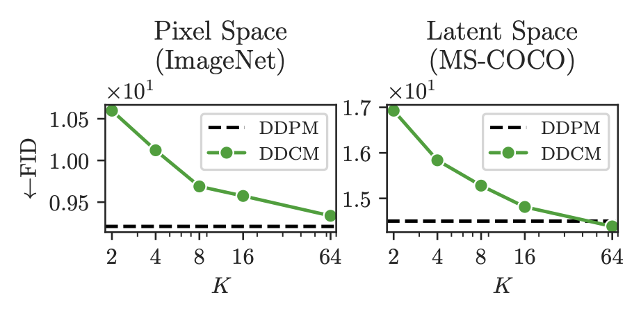Restricting the noise sampling space to a finite set does not noticeably worsen the FID of generated results

As we can see, by the time $K = 64$, the FID has essentially caught up; looking closely, one finds that even at $K=2$ the loss is minimal. This indicates that discretizing the sampling space largely preserves DDPM's generative capability. There's a subtlety worth noting here: the $\mathcal{C}_t$ at each step is independent, meaning that across all codebooks there are a total of $(T+1)K$ distinct noise vectors, rather than $K$ shared noise vectors. I did a simple reproduction and found that if the noise is shared across steps, you need $K\geq 8192$ to maintain comparable performance.

Discrete Coding

Now let's consider an inverse problem: given a target $\boldsymbol{x}_0$, find its discrete code, i.e., find the sequence $\boldsymbol{\varepsilon}_T\in \mathcal{C}_T,\cdots,\boldsymbol{\varepsilon}_1\in \mathcal{C}_1$ such that iterating via $\boldsymbol{x}_{t-1} = \boldsymbol{\mu}(\boldsymbol{x}_t) + \sigma_t \boldsymbol{\varepsilon}_t$ produces a $\boldsymbol{x}_0$ as close as possible to the given sample.

Since discretizing the sampling space doesn't noticeably change the FID, we can reasonably assume that all samples from the same distribution can theoretically be generated via equation $\eqref{eq:ddcm-g}$, so a solution to the inverse problem above should exist in principle. But how do we actually find it? The intuitive idea is to work backwards from $\boldsymbol{x}_0$, but on closer thought this turns out to be hard to operationalize — for instance, at the very first step, $\boldsymbol{x}_0 = \boldsymbol{\mu}(\boldsymbol{x}_1) + \sigma_1 \boldsymbol{\varepsilon}_1$, both $\boldsymbol{x}_1$ and $\boldsymbol{\varepsilon}_1$ are unknown, and it's difficult to pin them down simultaneously.

This is where DDCM's second flash of insight comes in: it treats the discrete coding of $\boldsymbol{x}_0$ as a conditional-control generation problem! Specifically, starting from a fixed $\boldsymbol{x}_T$, we select $\boldsymbol{\varepsilon}_t$ as follows:

\begin{equation}\boldsymbol{x}_{t-1} = \boldsymbol{\mu}(\boldsymbol{x}_t) + \sigma_t \boldsymbol{\varepsilon}_t,\quad \boldsymbol{\varepsilon}_t = \mathop{\text{argmax}}_{\boldsymbol{\varepsilon}\in\mathcal{C}_t} \boldsymbol{\varepsilon}\cdot(\boldsymbol{x}_0-\bar{\boldsymbol{\mu}}(\boldsymbol{x}_t))\label{eq:ddcm-eg}\end{equation}

Here $\bar{\boldsymbol{\mu}}(\boldsymbol{x}_t)$ is the model that predicts $\boldsymbol{x}_0$ from $\boldsymbol{x}_t$, related to $\boldsymbol{\mu}(\boldsymbol{x}_t)$ by:

\begin{equation}\boldsymbol{\mu}(\boldsymbol{x}_t) = \frac{\alpha_t\bar{\beta}_{t-1}^2}{\bar{\beta}_t^2}\boldsymbol{x}_t + \frac{\bar{\alpha}_{t-1}\beta_t^2}{\bar{\beta}_t^2}\bar{\boldsymbol{\mu}}(\boldsymbol{x}_t)\end{equation}

If readers have forgotten this part, they can revisit Diffusion Models Miscellany (3): DDPM = Bayes + Denoising for a refresher.

We'll leave the detailed derivation to the next section; for now, let's just look at equation $\eqref{eq:ddcm-eg}$. Its sole difference from the randomly-generated version, equation $\eqref{eq:ddcm-g}$, is that the optimal $\boldsymbol{\varepsilon}_t$ is chosen via $\text{argmax}$, with the criterion being the inner-product similarity between $\boldsymbol{\varepsilon}$ and the residual $\boldsymbol{x}_0-\bar{\boldsymbol{\mu}}(\boldsymbol{x}_t)$. Intuitively, this means choosing $\boldsymbol{\varepsilon}$ so as to compensate as much as possible for the current gap between $\bar{\boldsymbol{\mu}}(\boldsymbol{x}_t)$ and the target $\boldsymbol{x}_0$. By iterating equation $\eqref{eq:ddcm-eg}$, an image is equivalently converted into $T-1$ integers ($\sigma_1$ is usually set to zero).

The rule looks simple enough — but how well does it actually reconstruct images? Below is a figure taken from the original paper; the results are quite impressive, and there are more examples in the paper itself. I also tried this on my own model and found that I could basically reproduce similar results, so the method does appear to be reliable.

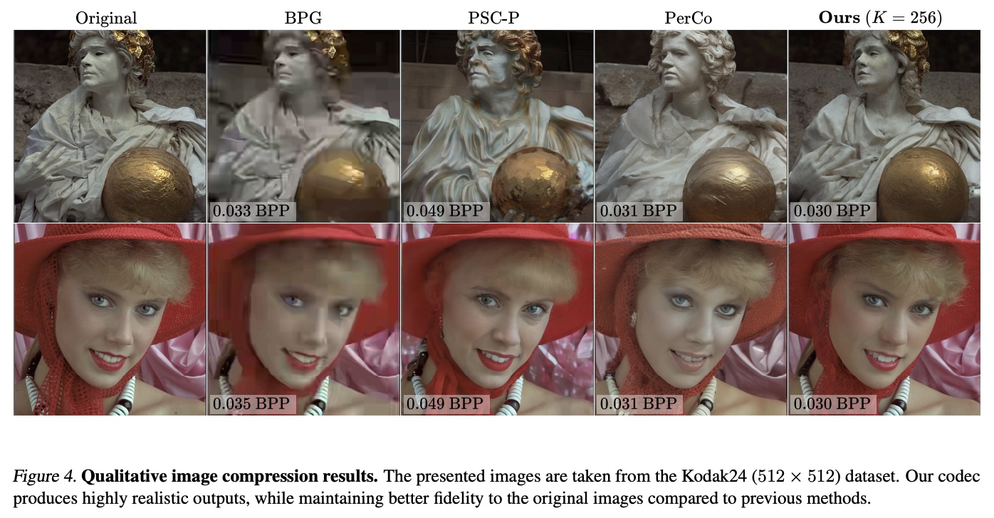DDCM's discrete-coding reconstruction results

Conditional Generation

We just said that DDCM treats the encoding process as a conditional-control generation process — what does that actually mean? Starting from DDPM's equation $\eqref{eq:ddpm-g}$, it can be equivalently written as

\begin{equation}p(\boldsymbol{x}_{t-1}|\boldsymbol{x}_t) = \mathcal{N}(\boldsymbol{x}_{t-1};\boldsymbol{\mu}(\boldsymbol{x}_t),\sigma_t^2\boldsymbol{I})\end{equation}

What we want to do now is control the generation process given knowledge of $\boldsymbol{x}_0$, so we add an extra condition $\boldsymbol{x}_0$ to the distribution above, changing it to $p(\boldsymbol{x}_{t-1}|\boldsymbol{x}_t,\boldsymbol{x}_0)$. In fact, within DDPM, $p(\boldsymbol{x}_{t-1}|\boldsymbol{x}_t,\boldsymbol{x}_0)$ has an analytical solution, which we already derived in Diffusion Models Miscellany (3): DDPM = Bayes + Denoising:

\begin{equation}p(\boldsymbol{x}_{t-1}|\boldsymbol{x}_t, \boldsymbol{x}_0) = \mathcal{N}\left(\boldsymbol{x}_{t-1};\frac{\alpha_t\bar{\beta}_{t-1}^2}{\bar{\beta}_t^2}\boldsymbol{x}_t + \frac{\bar{\alpha}_{t-1}\beta_t^2}{\bar{\beta}_t^2}\boldsymbol{x}_0,\frac{\bar{\beta}_{t-1}^2\beta_t^2}{\bar{\beta}_t^2} \boldsymbol{I}\right)\end{equation}

or equivalently,

\begin{equation}\begin{aligned} \boldsymbol{x}_{t-1} =&\, \frac{\alpha_t\bar{\beta}_{t-1}^2}{\bar{\beta}_t^2}\boldsymbol{x}_t + \frac{\bar{\alpha}_{t-1}\beta_t^2}{\bar{\beta}_t^2}\boldsymbol{x}_0 + \frac{\bar{\beta}_{t-1}\beta_t}{\bar{\beta}_t}\boldsymbol{\varepsilon}_t \\ =&\, \underbrace{\frac{\alpha_t\bar{\beta}_{t-1}^2}{\bar{\beta}_t^2}\boldsymbol{x}_t + \frac{\bar{\alpha}_{t-1}\beta_t^2}{\bar{\beta}_t^2}\bar{\boldsymbol{\mu}}(\boldsymbol{x}_t)}_{\boldsymbol{\mu}(\boldsymbol{x}_t)} + \frac{\bar{\alpha}_{t-1}\beta_t^2}{\bar{\beta}_t^2}(\boldsymbol{x}_0 - \bar{\boldsymbol{\mu}}(\boldsymbol{x}_t)) + \underbrace{\frac{\bar{\beta}_{t-1}\beta_t}{\bar{\beta}_t}}_{\sigma_t}\boldsymbol{\varepsilon}_t \end{aligned}\label{eq:ddcm-eg0}\end{equation}

where $\boldsymbol{\varepsilon}_t\sim\mathcal{N}(\boldsymbol{0},\boldsymbol{I})$. Compared with equation $\eqref{eq:ddpm-g}$, the equation above has an extra term $\boldsymbol{x}_0 - \bar{\boldsymbol{\mu}}(\boldsymbol{x}_t)$, which pulls the generation result toward $\boldsymbol{x}_0$. But recall that our task is discrete coding of $\boldsymbol{x}_0$, so the generation process must not explicitly involve $\boldsymbol{x}_0$ — otherwise we'd be putting the cart before the horse. To resolve this, we hope that the term $\boldsymbol{x}_0 - \bar{\boldsymbol{\mu}}(\boldsymbol{x}_t)$ can be compensated for by $\boldsymbol{\varepsilon}_t$, so we adjust the selection rule for $\boldsymbol{\varepsilon}_t$ to

\begin{equation}\boldsymbol{\varepsilon}_t = \mathop{\text{argmin}}_{\boldsymbol{\varepsilon}\in\mathcal{C}_t} \left\Vert\frac{\bar{\alpha}_{t-1}\beta_t^2}{\bar{\beta}_t^2}(\boldsymbol{x}_0 - \bar{\boldsymbol{\mu}}(\boldsymbol{x}_t)) - \frac{\bar{\beta}_{t-1}\beta_t}{\bar{\beta}_t}\boldsymbol{\varepsilon}\right\Vert\label{eq:ddcm-eps0}\end{equation}

Since the vectors in $\mathcal{C}_t$ are all pre-sampled from $\mathcal{N}(\boldsymbol{0},\boldsymbol{I})$, similarly to the "unit-norm lemma" from The Amazing Johnson–Lindenstrauss Lemma: Theory, we can assume that the vectors in $\mathcal{C}_t$ have roughly equal norms. Under this assumption, the equation above is also equivalent to

\begin{equation}\boldsymbol{\varepsilon}_t = \mathop{\text{argmax}}_{\boldsymbol{\varepsilon}\in\mathcal{C}_t} \boldsymbol{\varepsilon}\cdot(\boldsymbol{x}_0-\bar{\boldsymbol{\mu}}(\boldsymbol{x}_t))\end{equation}

and this gives us DDCM's equation $\eqref{eq:ddcm-eg}$.

Importance Sampling

In the derivation above, we invoked the claim that "we hope the term $\boldsymbol{x}_0 - \bar{\boldsymbol{\mu}}(\boldsymbol{x}_t)$ can be compensated for by $\boldsymbol{\varepsilon}_t$, so we change the selection rule for $\boldsymbol{\varepsilon}_t$ to equation $\eqref{eq:ddcm-eps0}$." While this sounds intuitive, it is not rigorous mathematically — indeed, strictly speaking, it's incorrect. In this section we'll make this rigorous.

Let's revisit equation $\eqref{eq:ddcm-eg0}$ again. The derivation up through equation $\eqref{eq:ddcm-eg0}$ is rigorous; what's not rigorous is the way we connect equation $\eqref{eq:ddcm-eg0}$ to $\mathcal{C}_t$. Consider: if we select $\boldsymbol{\varepsilon}_t$ according to $\eqref{eq:ddcm-eps0}$, what happens as $K\to\infty$? At that point we can say that $\mathcal{C}_t$ has essentially covered the entirety of $\mathbb{R}^d$, so $\frac{\bar{\alpha}_{t-1}\beta_t^2}{\bar{\beta}_t^2}(\boldsymbol{x}_0 - \bar{\boldsymbol{\mu}}(\boldsymbol{x}_t)) = \frac{\bar{\beta}_{t-1}\beta_t}{\bar{\beta}_t}\boldsymbol{\varepsilon}_t$ — meaning equation $\eqref{eq:ddcm-eg0}$ becomes a deterministic transformation:

\begin{equation}\boldsymbol{x}_{t-1} = \frac{\alpha_t\bar{\beta}_{t-1}^2}{\bar{\beta}_t^2}\boldsymbol{x}_t + \frac{\bar{\alpha}_{t-1}\beta_t^2}{\bar{\beta}_t^2}\bar{\boldsymbol{\mu}}(\boldsymbol{x}_t) + \frac{\bar{\alpha}_{t-1}\beta_t^2}{\bar{\beta}_t^2}(\boldsymbol{x}_0 - \bar{\boldsymbol{\mu}}(\boldsymbol{x}_t)) = \frac{\alpha_t\bar{\beta}_{t-1}^2}{\bar{\beta}_t^2}\boldsymbol{x}_t + \frac{\bar{\alpha}_{t-1}\beta_t^2}{\bar{\beta}_t^2}\boldsymbol{x}_0\end{equation}

In other words, when $K\to\infty$, we can no longer recover the original random sampling trajectory, which is not really a scientifically sound outcome. We'd argue that discretizing the sampling space should be viewed as an approximation to the continuous sampling space, and that as $K\to\infty$, it should recover the continuous sampling trajectory — only then does each discretized step have a proper theoretical guarantee. Put more mathematically, we consider it a necessary condition that

\begin{equation}\lim_{K\to\infty} \text{DDCM} = \text{DDPM}\end{equation}

Going from equation $\eqref{eq:ddpm-g}$ to equation $\eqref{eq:ddcm-eg0}$, we can also think of this as switching the noise distribution from $\mathcal{N}(\boldsymbol{0},\boldsymbol{I})$ to $\mathcal{N}(\frac{\bar{\alpha}_{t-1}\beta_t^2}{\bar{\beta}_t^2\sigma_t}(\boldsymbol{x}_0 - \bar{\boldsymbol{\mu}}(\boldsymbol{x}_t)),\boldsymbol{I})$; but because of the requirements of coding, we cannot sample directly from the latter — we can only sample from the finite set $\mathcal{C}_t$. To satisfy the necessary condition, i.e., to make the sampled result closer to sampling from $\mathcal{N}(\frac{\bar{\alpha}_{t-1}\beta_t^2}{\bar{\beta}_t^2\sigma_t}(\boldsymbol{x}_0 - \bar{\boldsymbol{\mu}}(\boldsymbol{x}_t)),\boldsymbol{I})$, we can weight $\boldsymbol{\varepsilon}\in\mathcal{C}_t$ using its probability density function:

\begin{equation}p(\boldsymbol{\varepsilon})\propto \exp\left(-\frac{1}{2}\left\Vert\boldsymbol{\varepsilon} - \frac{\bar{\alpha}_{t-1}\beta_t^2}{\bar{\beta}_t^2\sigma_t}(\boldsymbol{x}_0 - \bar{\boldsymbol{\mu}}(\boldsymbol{x}_t))\right\Vert^2\right),\quad \boldsymbol{\varepsilon}\in\mathcal{C}_t\label{eq:ddcm-p}\end{equation}

That is to say, the most sensible approach should be to apply a softmax to $-\frac{1}{2}\left\Vert\boldsymbol{\varepsilon} - \frac{\bar{\alpha}_{t-1}\beta_t^2}{\bar{\beta}_t^2\sigma_t}(\boldsymbol{x}_0 - \bar{\boldsymbol{\mu}}(\boldsymbol{x}_t))\right\Vert^2$ and then perform importance sampling according to the resulting probabilities, rather than simply taking the argmax $\text{argmax}$. It's just that when $K$ is relatively small, the distribution after softmax approaches a one-hot distribution, so sampling by probability becomes roughly equivalent to taking $\text{argmax}$.

General Form

We can also generalize the above result to classifier-guidance generation. Following the derivation in Diffusion Models Miscellany (9): Conditional Control of Generated Results, adding classifier guidance to equation $\eqref{eq:ddpm-g}$ gives

\begin{equation}\boldsymbol{x}_{t-1} = \boldsymbol{\mu}(\boldsymbol{x}_t) + \sigma_t^2 \nabla_{\boldsymbol{x}_t} \log p(\boldsymbol{y}|\boldsymbol{x}_t) + \sigma_t\boldsymbol{\varepsilon}_t,\quad \boldsymbol{\varepsilon}_t\sim \mathcal{N}(\boldsymbol{0},\boldsymbol{I})\end{equation}

i.e., we add a new term $\sigma_t^2 \nabla_{\boldsymbol{x}_t} \log p(\boldsymbol{y}|\boldsymbol{x}_t)$, where $p(\boldsymbol{y}|\boldsymbol{x}_t)$ is a classifier operating on noisy samples. If we only have a classifier on noise-free samples $p_o(\boldsymbol{y}|\boldsymbol{x})$, we can also let $p(\boldsymbol{y}|\boldsymbol{x}_t) = p_{o}(\boldsymbol{y}|\boldsymbol{\mu}(\boldsymbol{x}_t))$.

Following the same reasoning, we can obtain a selection rule analogous to equation $\eqref{eq:ddcm-eps0}$:

\begin{equation}\boldsymbol{\varepsilon}_t = \mathop{\text{argmin}}_{\boldsymbol{\varepsilon}\in\mathcal{C}_t} \left\Vert\sigma_t^2 \nabla_{\boldsymbol{x}_t} \log p(\boldsymbol{y}|\boldsymbol{x}_t) - \sigma_t\boldsymbol{\varepsilon}\right\Vert\end{equation}

or approximately,

\begin{equation}\boldsymbol{\varepsilon}_t = \mathop{\text{argmax}}_{\boldsymbol{\varepsilon}\in\mathcal{C}_t} \boldsymbol{\varepsilon}\cdot\nabla_{\boldsymbol{x}_t} \log p(\boldsymbol{y}|\boldsymbol{x}_t)\end{equation}

Of course, we could also construct a sampling distribution following equation $\eqref{eq:ddcm-p}$:

\begin{equation}p(\boldsymbol{\varepsilon})\propto \exp\left(-\frac{1}{2}\left\Vert\boldsymbol{\varepsilon} - \sigma_t\nabla_{\boldsymbol{x}_t} \log p(\boldsymbol{y}|\boldsymbol{x}_t)\right\Vert^2\right),\quad \boldsymbol{\varepsilon}\in\mathcal{C}_t\end{equation}

These are all just simple generalizations of the results derived earlier.

Personal Commentary

At this point, we've essentially finished introducing DDCM; for further details, readers should consult the original paper. The authors haven't released their code yet, so here I offer my own reference implementation:

DDCM: https://github.com/bojone/Keras-DDPM/blob/main/ddcm.py

If you already have some familiarity with diffusion models and have a working diffusion model on hand, I strongly recommend trying this out yourself. The underlying principle of DDCM is quite easy to grasp, and the code isn't hard to write — but only by trying it firsthand can you really experience that jaw-dropping sense of amazement. The last time I had a similar feeling was with Upsample Guidance, the training-free technique for generating large images introduced in Diffusion Models Miscellany (23): Signal-to-Noise Ratio and Large-Image Generation (Part 2) — it likewise reflected a truly original piece of thinking on the author's part.

That said, in terms of long-term impact, I personally think Upsample Guidance is still not quite on the level of DDCM. This is because discretizing images into codes is one of the mainstream approaches in multimodal LLMs, serving as an "image tokenizer" — a rather crucial component — and DDCM can be said to have opened up an entirely new path alongside VQ and FSQ, which means it may end up having a much more far-reaching influence. In the original paper, DDCM is framed merely as a compression method, which, if anything, seems to undersell it.

As a discrete coding model, DDCM has another particularly striking advantage: the discrete codes it produces are naturally 1D, unlike schemes such as VQ and FSQ, whose encoded results typically retain the image's 2D structure (with the exception of models like TiTok, which borrow ideas from Q-Former to convert to 1D). This means that when using these codes for autoregressive generation, we no longer need to worry about the "ordering" problem (see "Reinventing the Wheel" on Multimodality (2): Autoregression) — which is a considerable relief.

Of course, there's still room for improvement at present. For instance, currently encoding and generation happen simultaneously, meaning that however slow DDPM's sampling is, DDCM's encoding is equally slow — which, at present, isn't really acceptable. And unfortunately we can't simply apply accelerated-sampling tricks here, because accelerating sampling means reducing $T$, and reducing $T$ means shortening the code length, i.e., increasing the compression ratio — which would noticeably increase the reconstruction loss.

All told, I think DDCM is a genuinely fascinating discrete-coding method, one with plenty of untapped potential that also urgently calls for further optimization.

Summary

This post introduced a new twist on diffusion models: by restricting the noise used in DDPM's generation process to a finite set, and combining this with ideas from conditional generation, one can turn a DDPM, without any additional training, into something akin to a VQ-VAE discrete autoencoder.