Generative Diffusion Models Explained (III): DDPM = Bayes + Denoising

生成扩散模型漫谈（三）：DDPM = 贝叶斯 + 去噪 苏剑林 · 2022-07-19 · Machine Learning probability generative model DDPM diffusion

So far, I have presented two derivations of the generative diffusion model DDPM: the intuitive analogy approach in Generative Diffusion Models Explained (I): DDPM = Demolishing Buildings + Building Buildings, and the variational autoencoder approach in Generative Diffusion Models Explained (II): DDPM = Autoregressive VAE. Each has its own strengths: the former is more intuitive and easy to grasp, but doesn't lend itself to further theoretical extension or quantitative understanding; the latter is more complete in its theoretical analysis, but is somewhat formalistic and less illuminating.

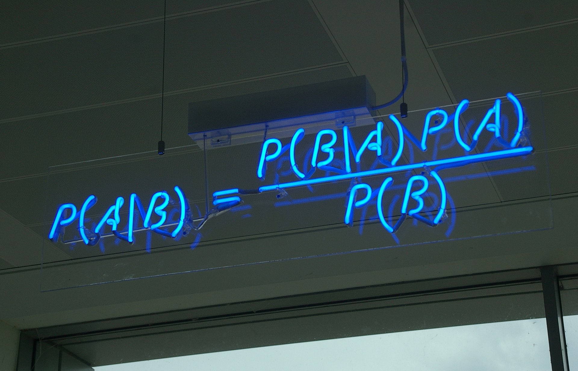Bayes' theorem (from Wikipedia)

In this article, I'll share yet another derivation of DDPM, one that makes heavy use of Bayes' theorem to simplify the calculations. The whole process has a strong flavor of "working things out step by step," and is quite illuminating. Moreover, it is closely connected to the DDIM model that we'll introduce later. more

Setting the Scene

Let's again recall the transformation process modeled by DDPM:

\begin{equation}\boldsymbol{x} = \boldsymbol{x}_0 \rightleftharpoons \boldsymbol{x}_1 \rightleftharpoons \boldsymbol{x}_2 \rightleftharpoons \cdots \rightleftharpoons \boldsymbol{x}_{T-1} \rightleftharpoons \boldsymbol{x}_T = \boldsymbol{z}\end{equation}

Here, the forward process gradually turns sample data $\boldsymbol{x}$ into random noise $\boldsymbol{z}$, while the reverse process gradually turns random noise $\boldsymbol{z}$ back into sample data $\boldsymbol{x}$. The reverse process is the "generative model" we're after.

The forward process is simple; each step is

\begin{equation}\boldsymbol{x}_t = \alpha_t \boldsymbol{x}_{t-1} + \beta_t \boldsymbol{\varepsilon}_t,\quad \boldsymbol{\varepsilon}_t\sim\mathcal{N}(\boldsymbol{0}, \boldsymbol{I})\end{equation}

or equivalently $p(\boldsymbol{x}_t|\boldsymbol{x}_{t-1})=\mathcal{N}(\boldsymbol{x}_t;\alpha_t \boldsymbol{x}_{t-1},\beta_t^2 \boldsymbol{I})$. Under the constraint $\alpha_t^2 + \beta_t^2 = 1$, we have

\begin{equation}\begin{aligned} \boldsymbol{x}_t =&\, \alpha_t \boldsymbol{x}_{t-1} + \beta_t \boldsymbol{\varepsilon}_t \\ =&\, \alpha_t \big(\alpha_{t-1} \boldsymbol{x}_{t-2} + \beta_{t-1} \boldsymbol{\varepsilon}_{t-1}\big) + \beta_t \boldsymbol{\varepsilon}_t \\ =&\,\cdots\\ =&\,(\alpha_t\cdots\alpha_1) \boldsymbol{x}_0 + \underbrace{(\alpha_t\cdots\alpha_2)\beta_1 \boldsymbol{\varepsilon}_1 + (\alpha_t\cdots\alpha_3)\beta_2 \boldsymbol{\varepsilon}_2 + \cdots + \alpha_t\beta_{t-1} \boldsymbol{\varepsilon}_{t-1} + \beta_t \boldsymbol{\varepsilon}_t}_{\sim \mathcal{N}(\boldsymbol{0}, (1-\alpha_t^2\cdots\alpha_1^2)\boldsymbol{I})} \end{aligned}\end{equation}

from which we can derive $p(\boldsymbol{x}_t|\boldsymbol{x}_0)=\mathcal{N}(\boldsymbol{x}_t;\bar{\alpha}_t \boldsymbol{x}_0,\bar{\beta}_t^2 \boldsymbol{I})$, where $\bar{\alpha}_t = \alpha_1\cdots\alpha_t$ and $\bar{\beta}_t = \sqrt{1-\bar{\alpha}_t^2}$.

What DDPM needs to do is to derive $p(\boldsymbol{x}_{t-1}|\boldsymbol{x}_t)$, which is needed for the reverse process, from the above information. This would let us start from an arbitrary $\boldsymbol{x}_T=\boldsymbol{z}$, sample step by step to get $\boldsymbol{x}_{T-1},\boldsymbol{x}_{T-2},\cdots,\boldsymbol{x}_1$, and finally obtain a randomly generated sample $\boldsymbol{x}_0=\boldsymbol{x}$.

Enter Bayes

Now let's bring in the great Bayes' theorem. In fact, applying Bayes' theorem directly, we have

\begin{equation}p(\boldsymbol{x}_{t-1}|\boldsymbol{x}_t) = \frac{p(\boldsymbol{x}_t|\boldsymbol{x}_{t-1})p(\boldsymbol{x}_{t-1})}{p(\boldsymbol{x}_t)}\label{eq:bayes}\end{equation}

However, we don't know the expression for $p(\boldsymbol{x}_{t-1}),p(\boldsymbol{x}_t)$, so this route is a dead end. But we can settle for the next best thing: apply Bayes' theorem conditioned on $\boldsymbol{x}_0$:

\begin{equation}p(\boldsymbol{x}_{t-1}|\boldsymbol{x}_t, \boldsymbol{x}_0) = \frac{p(\boldsymbol{x}_t|\boldsymbol{x}_{t-1})p(\boldsymbol{x}_{t-1}|\boldsymbol{x}_0)}{p(\boldsymbol{x}_t|\boldsymbol{x}_0)}\end{equation}

We make this modification precisely because $p(\boldsymbol{x}_t|\boldsymbol{x}_{t-1}),p(\boldsymbol{x}_{t-1}|\boldsymbol{x}_0),p(\boldsymbol{x}_t|\boldsymbol{x}_0)$ are all known, so the expression above is computable. Substituting in their respective forms, we get:

\begin{equation}p(\boldsymbol{x}_{t-1}|\boldsymbol{x}_t, \boldsymbol{x}_0) = \mathcal{N}\left(\boldsymbol{x}_{t-1};\frac{\alpha_t\bar{\beta}_{t-1}^2}{\bar{\beta}_t^2}\boldsymbol{x}_t + \frac{\bar{\alpha}_{t-1}\beta_t^2}{\bar{\beta}_t^2}\boldsymbol{x}_0,\frac{\bar{\beta}_{t-1}^2\beta_t^2}{\bar{\beta}_t^2} \boldsymbol{I}\right)\label{eq:p-xt-x0}\end{equation}

Derivation:
The derivation above isn't difficult — it's just routine expansion and rearrangement, though we can use a few tricks to speed things up. First, substituting in the respective expressions, we find that, apart from the $-1/2$ factor, the exponent works out to:
\begin{equation}\frac{\Vert \boldsymbol{x}_t - \alpha_t \boldsymbol{x}_{t-1}\Vert^2}{\beta_t^2} + \frac{\Vert \boldsymbol{x}_{t-1} - \bar{\alpha}_{t-1}\boldsymbol{x}_0\Vert^2}{\bar{\beta}_{t-1}^2} - \frac{\Vert \boldsymbol{x}_t - \bar{\alpha}_t \boldsymbol{x}_0\Vert^2}{\bar{\beta}_t^2}\end{equation}
Since this is quadratic in $\boldsymbol{x}_{t-1}$, the resulting distribution must also be Gaussian, so we only need to find its mean and covariance. It's easy to see that the coefficient of the $\Vert \boldsymbol{x}_{t-1}\Vert^2$ term in the expansion is
\begin{equation}\frac{\alpha_t^2}{\beta_t^2} + \frac{1}{\bar{\beta}_{t-1}^2} = \frac{\alpha_t^2\bar{\beta}_{t-1}^2 + \beta_t^2}{\bar{\beta}_{t-1}^2 \beta_t^2} = \frac{\alpha_t^2(1-\bar{\alpha}_{t-1}^2) + \beta_t^2}{\bar{\beta}_{t-1}^2 \beta_t^2} = \frac{1-\bar{\alpha}_t^2}{\bar{\beta}_{t-1}^2 \beta_t^2} = \frac{\bar{\beta}_t^2}{\bar{\beta}_{t-1}^2 \beta_t^2}\end{equation}
so the tidied-up result must take the form $\frac{\bar{\beta}_t^2}{\bar{\beta}_{t-1}^2 \beta_t^2}\Vert \boldsymbol{x}_{t-1} - \tilde{\boldsymbol{\mu}}(\boldsymbol{x}_t, \boldsymbol{x}_0)\Vert^2$, which means the covariance matrix is $\frac{\bar{\beta}_{t-1}^2 \beta_t^2}{\bar{\beta}_t^2}\boldsymbol{I}$. On the other hand, pulling out the coefficient of the linear term gives $-2\left(\frac{\alpha_t}{\beta_t^2}\boldsymbol{x}_t + \frac{\bar{\alpha}_{t-1}}{\bar{\beta}_{t-1}^2}\boldsymbol{x}_0 \right)$, and dividing by $\frac{-2\bar{\beta}_t^2}{\bar{\beta}_{t-1}^2 \beta_t^2}$ yields
\begin{equation}\tilde{\boldsymbol{\mu}}(\boldsymbol{x}_t, \boldsymbol{x}_0)=\frac{\alpha_t\bar{\beta}_{t-1}^2}{\bar{\beta}_t^2}\boldsymbol{x}_t + \frac{\bar{\alpha}_{t-1}\beta_t^2}{\bar{\beta}_t^2}\boldsymbol{x}_0 \end{equation}
This gives us all the information we need about $p(\boldsymbol{x}_{t-1}|\boldsymbol{x}_t, \boldsymbol{x}_0)$, and the result is exactly equation $\eqref{eq:p-xt-x0}$.

The Denoising Process

We have now obtained $p(\boldsymbol{x}_{t-1}|\boldsymbol{x}_t, \boldsymbol{x}_0)$, which has an explicit solution — but it is not yet the final answer we want, because we only want to predict $\boldsymbol{x}_{t-1}$ from $\boldsymbol{x}_t$, without relying on $\boldsymbol{x}_0$, since $\boldsymbol{x}_0$ is precisely what we ultimately want to generate. This brings us to a somewhat "wild" idea:

If we could predict $\boldsymbol{x}_0$ from $\boldsymbol{x}_t$, couldn't we then eliminate the $\boldsymbol{x}_0$ inside $p(\boldsymbol{x}_{t-1}|\boldsymbol{x}_t, \boldsymbol{x}_0)$, making it depend only on $\boldsymbol{x}_t$?

No sooner said than done: we use $\bar{\boldsymbol{\mu}}(\boldsymbol{x}_t)$ to estimate $\boldsymbol{x}_0$, with loss function $\Vert \boldsymbol{x}_0 - \bar{\boldsymbol{\mu}}(\boldsymbol{x}_t)\Vert^2$. Once trained, we take it that

\begin{equation}p(\boldsymbol{x}_{t-1}|\boldsymbol{x}_t) \approx p(\boldsymbol{x}_{t-1}|\boldsymbol{x}_t, \boldsymbol{x}_0=\bar{\boldsymbol{\mu}}(\boldsymbol{x}_t)) = \mathcal{N}\left(\boldsymbol{x}_{t-1}; \frac{\alpha_t\bar{\beta}_{t-1}^2}{\bar{\beta}_t^2}\boldsymbol{x}_t + \frac{\bar{\alpha}_{t-1}\beta_t^2}{\bar{\beta}_t^2}\bar{\boldsymbol{\mu}}(\boldsymbol{x}_t),\frac{\bar{\beta}_{t-1}^2\beta_t^2}{\bar{\beta}_t^2} \boldsymbol{I}\right)\label{eq:p-xt}\end{equation}

In $\Vert \boldsymbol{x}_0 - \bar{\boldsymbol{\mu}}(\boldsymbol{x}_t)\Vert^2$, $\boldsymbol{x}_0$ represents the original data and $\boldsymbol{x}_t$ represents the noisy data, so this is in effect training a denoising model — which is exactly what the first "D" in DDPM stands for (Denoising).

Concretely, $p(\boldsymbol{x}_t|\boldsymbol{x}_0)=\mathcal{N}(\boldsymbol{x}_t;\bar{\alpha}_t \boldsymbol{x}_0,\bar{\beta}_t^2 \boldsymbol{I})$ implies $\boldsymbol{x}_t = \bar{\alpha}_t \boldsymbol{x}_0 + \bar{\beta}_t \boldsymbol{\varepsilon},\boldsymbol{\varepsilon}\sim\mathcal{N}(\boldsymbol{0}, \boldsymbol{I})$, or equivalently $\boldsymbol{x}_0 = \frac{1}{\bar{\alpha}_t}\left(\boldsymbol{x}_t - \bar{\beta}_t \boldsymbol{\varepsilon}\right)$, which suggests parameterizing $\bar{\boldsymbol{\mu}}(\boldsymbol{x}_t)$ as

\begin{equation}\bar{\boldsymbol{\mu}}(\boldsymbol{x}_t) = \frac{1}{\bar{\alpha}_t}\left(\boldsymbol{x}_t - \bar{\beta}_t \boldsymbol{\epsilon}_{\boldsymbol{\theta}}(\boldsymbol{x}_t, t)\right)\label{eq:bar-mu}\end{equation}

At this point the loss function becomes

\begin{equation}\Vert \boldsymbol{x}_0 - \bar{\boldsymbol{\mu}}(\boldsymbol{x}_t)\Vert^2 = \frac{\bar{\beta}_t^2}{\bar{\alpha}_t^2}\left\Vert\boldsymbol{\varepsilon} - \boldsymbol{\epsilon}_{\boldsymbol{\theta}}(\bar{\alpha}_t \boldsymbol{x}_0 + \bar{\beta}_t \boldsymbol{\varepsilon}, t)\right\Vert^2\end{equation}

Dropping the leading coefficient, we arrive at exactly the loss function used in the original DDPM paper. Notice that this article derives the denoising process from $\boldsymbol{x}_t$ to $\boldsymbol{x}_0$ directly, rather than going through the denoising process from $\boldsymbol{x}_t$ to $\boldsymbol{x}_{t-1}$ plus an integral transform, as in the previous two articles. In comparison, the derivation here gets there in one step.

On the other hand, substituting equation $\eqref{eq:bar-mu}$ into equation $\eqref{eq:p-xt}$ and simplifying, we get

\begin{equation} p(\boldsymbol{x}_{t-1}|\boldsymbol{x}_t) \approx p(\boldsymbol{x}_{t-1}|\boldsymbol{x}_t, \boldsymbol{x}_0=\bar{\boldsymbol{\mu}}(\boldsymbol{x}_t)) = \mathcal{N}\left(\boldsymbol{x}_{t-1}; \frac{1}{\alpha_t}\left(\boldsymbol{x}_t - \frac{\beta_t^2}{\bar{\beta}_t}\boldsymbol{\epsilon}_{\boldsymbol{\theta}}(\boldsymbol{x}_t, t)\right),\frac{\bar{\beta}_{t-1}^2\beta_t^2}{\bar{\beta}_t^2} \boldsymbol{I}\right)\end{equation}

This is the distribution used for the reverse sampling process, and it also pins down the variance used in sampling. That completes the derivation of DDPM. (Note: for the sake of a smoother derivation, the $\boldsymbol{\epsilon}_{\boldsymbol{\theta}}$ used here differs from the previous two articles, and instead matches the original DDPM paper.)

Derivation:
Substituting equation $\eqref{eq:bar-mu}$ into equation $\eqref{eq:p-xt}$, the main difficulty in simplifying lies in computing
\begin{equation}\begin{aligned}\frac{\alpha_t\bar{\beta}_{t-1}^2}{\bar{\beta}_t^2} + \frac{\bar{\alpha}_{t-1}\beta_t^2}{\bar{\alpha}_t\bar{\beta}_t^2} =&\, \frac{\alpha_t\bar{\beta}_{t-1}^2 + \beta_t^2/\alpha_t}{\bar{\beta}_t^2} = \frac{\alpha_t^2(1-\bar{\alpha}_{t-1}^2) + \beta_t^2}{\alpha_t\bar{\beta}_t^2} = \frac{1-\bar{\alpha}_t^2}{\alpha_t\bar{\beta}_t^2} = \frac{1}{\alpha_t} > \end{aligned}\end{equation}

Predictor-Corrector

I wonder if readers have noticed something interesting here: what we're trying to do is gradually turn $\boldsymbol{x}_T$ into $\boldsymbol{x}_0$, yet in approximating $p(\boldsymbol{x}_{t-1}|\boldsymbol{x}_t)$ with $p(\boldsymbol{x}_{t-1}|\boldsymbol{x}_t, \boldsymbol{x}_0)$, we've included a step of "using $\bar{\boldsymbol{\mu}}(\boldsymbol{x}_t)$ to estimate $\boldsymbol{x}_0$." If that estimate were accurate, couldn't we just get there in one step — why bother with step-by-step sampling at all?

The reality is that "using $\bar{\boldsymbol{\mu}}(\boldsymbol{x}_t)$ to estimate $\boldsymbol{x}_0$" is of course not very accurate — at least not for a good many of the early steps. It merely serves as a forward-looking estimate, and we only use $p(\boldsymbol{x}_{t-1}|\boldsymbol{x}_t)$ to advance a small step. This is exactly the "predictor-corrector" idea found in many numerical algorithms: we use a rough solution to project far ahead, and then use that rough result to advance the final result by just a small step, gradually obtaining a more refined solution.

This brings to mind the Lookahead Optimizer: k steps forward, 1 step back, proposed by Hinton three years ago, which likewise consists of a prediction part (k steps forward) and a correction part (1 step back). The original paper frames this as a combination of "fast" and "slow" weights, where the fast weights are the predicted result and the slow weights are the corrected result based on that prediction. If we like, we can interpret DDPM's "predict-correct" process in exactly the same way.

An Unfinished Question

Finally, in the section on applying Bayes' theorem, we noted that equation $\eqref{eq:bayes}$ can't be used directly because neither $p(\boldsymbol{x}_{t-1})$ nor $p(\boldsymbol{x}_t)$ is known. By definition, we have

\begin{equation}p(\boldsymbol{x}_t) = \int p(\boldsymbol{x}_t|\boldsymbol{x}_0)\tilde{p}(\boldsymbol{x}_0)d\boldsymbol{x}_0\end{equation}

where $p(\boldsymbol{x}_t|\boldsymbol{x}_0)$ is known, but the data distribution $\tilde{p}(\boldsymbol{x}_0)$ cannot be known in advance, so this cannot be computed. However, there are two special cases in which both can be computed directly, which we'll work through here — and the results happen to answer the question about the choice of variance left open in the previous article.

The first example is when the entire dataset consists of a single sample. Without loss of generality, suppose this sample is $\boldsymbol{0}$; then $\tilde{p}(\boldsymbol{x}_0)$ is the Dirac distribution $\delta(\boldsymbol{x}_0)$, and we can directly compute $p(\boldsymbol{x}_t)=p(\boldsymbol{x}_t|\boldsymbol{0})$. Substituting into equation $\eqref{eq:bayes}$, we find the result is exactly the special case of $p(\boldsymbol{x}_{t-1}|\boldsymbol{x}_t,\boldsymbol{x}_0)$ with $\boldsymbol{x}_0=\boldsymbol{0}$, i.e.,

\begin{equation}p(\boldsymbol{x}_{t-1}|\boldsymbol{x}_t) = p(\boldsymbol{x}_{t-1}|\boldsymbol{x}_t, \boldsymbol{x}_0=\boldsymbol{0}) = \mathcal{N}\left(\boldsymbol{x}_{t-1};\frac{\alpha_t\bar{\beta}_{t-1}^2}{\bar{\beta}_t^2}\boldsymbol{x}_t,\frac{\bar{\beta}_{t-1}^2\beta_t^2}{\bar{\beta}_t^2} \boldsymbol{I}\right)\end{equation}

We're mainly interested in its variance, $\frac{\bar{\beta}_{t-1}^2\beta_t^2}{\bar{\beta}_t^2}$, which gives one choice for the sampling variance.

The second example is when the dataset follows a standard normal distribution, i.e., $\tilde{p}(\boldsymbol{x}_0)=\mathcal{N}(\boldsymbol{x}_0;\boldsymbol{0},\boldsymbol{I})$. Earlier we noted that $p(\boldsymbol{x}_t|\boldsymbol{x}_0)=\mathcal{N}(\boldsymbol{x}_t;\bar{\alpha}_t \boldsymbol{x}_0,\bar{\beta}_t^2 \boldsymbol{I})$ implies $\boldsymbol{x}_t = \bar{\alpha}_t \boldsymbol{x}_0 + \bar{\beta}_t \boldsymbol{\varepsilon},\boldsymbol{\varepsilon}\sim\mathcal{N}(\boldsymbol{0}, \boldsymbol{I})$, and by assumption here we also have $\boldsymbol{x}_0\sim\mathcal{N}(\boldsymbol{0}, \boldsymbol{I})$, so by the additivity of Gaussians, $\boldsymbol{x}_t$ also follows a standard normal distribution. Substituting the density of the standard normal distribution into equation $\eqref{eq:bayes}$, apart from the $-1/2$ factor, the exponent works out to:

\begin{equation}\frac{\Vert \boldsymbol{x}_t - \alpha_t \boldsymbol{x}_{t-1}\Vert^2}{\beta_t^2} + \Vert \boldsymbol{x}_{t-1}\Vert^2 - \Vert \boldsymbol{x}_t\Vert^2\end{equation}

Following a process similar to the derivation of $p(\boldsymbol{x}_{t-1}|\boldsymbol{x}_t,\boldsymbol{x}_0)$, we find that this exponent corresponds to

\begin{equation}p(\boldsymbol{x}_{t-1}|\boldsymbol{x}_t) = \mathcal{N}\left(\boldsymbol{x}_{t-1};\alpha_t\boldsymbol{x}_t,\beta_t^2 \boldsymbol{I}\right)\end{equation}

Again, we're mainly interested in its variance, $\beta_t^2$, which gives another choice for the sampling variance.

Summary

This article presented a derivation of DDPM with a strong flavor of "working things out step by step," using Bayes' theorem to directly derive the reverse generative process. Compared with the earlier "demolish-and-rebuild" analogy and the variational inference perspective, this derivation gets there more directly, in one step. It is also more illuminating, and closely connected to the DDIM model we'll introduce next.