The Embarrassingly Simple FSQ: "Rounding" Outperforms VQ-VAE
Just like "XXX is all you need," a fair number of papers are named "An Embarrassingly Simple XXX," but in my view, most of these papers deliver more hype than substance. However, a paper I recently read genuinely made me exclaim "embarrassingly simple" without any irony.
The paper is titled Finite Scalar Quantization: VQ-VAE Made Simple]. As the name suggests, this is a piece of work aimed at simplifying VQ-VAE with FSQ (Finite Scalar Quantization). As generative models and multimodal LLMs have grown increasingly popular, VQ-VAE and its follow-up works have likewise risen in prominence as an "image tokenizer." However, training VQ-VAE itself comes with certain issues, and this FSQ paper claims that a much simpler "rounding" operation can achieve the same goal—while also converging faster, training more stably, and producing better results.
Is FSQ really that magical? Let's find out together.
VQ
First, let's get familiar with "VQ." VQ stands for "Vector Quantize," which can be translated as "vector quantization"—a technique for mapping infinite, continuous encoding vectors to a finite set of discrete integers. If we apply VQ to the intermediate layer of an autoencoder, we can compress the size of the input while turning the encoding result into a discrete sequence of integers. more
Assuming the autoencoder's reconstruction loss is satisfactory, this integer sequence becomes an equivalent representation of the original image, and all operations on the original image can be converted into operations on the integer sequence. For instance, if we want to train an image generation model, we only need to train an integer-sequence generation model—which is equivalent to text generation. This means we can use it to train a GPT, with the same model and pipeline as for text. Once trained, we can sample integer sequences from the GPT model and feed them into the decoder to obtain images, thereby completing the construction of an image generation model. In short, "VQ + autoencoder" converts any input into an integer sequence consistent with text, unifying the input format across different modalities of data, and, at the same time, unifying their processing and generative models.
Such an autoencoder equipped with VQ functionality is called "VQ-VAE."
AE
Back in an article from four years ago, A Concise Introduction to VQ-VAE: The Quantized Autoencoder], we already introduced VQ-VAE. Despite being labeled "VAE (Variational AutoEncoder)," it actually has little to do with VAE—as mentioned in the previous section, it's simply an AE (AutoEncoder) equipped with VQ functionality.
Since it's an AE, it has an encoder and a decoder. An ordinary AE looks like this:
\begin{equation}z = encoder(x),\quad \hat{x}=decoder(z),\quad \mathcal{L}=\Vert x - \hat{x}\Vert^2 \end{equation}
VQ-VAE is slightly more complex:
\begin{equation}\begin{aligned} z =&\, encoder(x)\\[5pt] z_q =&\, z + \text{sg}[e_k - z],\quad k = \mathop{\text{argmin}}_{i\in\{1,2,\cdots,K\}} \Vert z - e_i\Vert\\ \hat{x} =&\, decoder(z_q)\\[5pt] \mathcal{L} =&\, \Vert x - \hat{x}\Vert^2 + \beta\Vert e_k - \text{sg}[z]\Vert^2 + \gamma\Vert z - \text{sg}[e_k]\Vert^2 \end{aligned}\label{eq:vqvae}\end{equation}
Let's walk through this step by step. First, the initial step is the same: the input $x$ goes into the encoder, which outputs the encoding vector $z$. However, we don't feed $z$ directly into the decoder. Instead, we first maintain a codebook of encoding vectors $\{e_1,e_2,\cdots,e_K\}$ (Codebook), from which we select the entry $e_k$ closest to $z$ and feed it into the decoder for reconstruction $x$. Since the codebook is finite, we can also understand the actual encoding result as an integer (namely, the index $k$ of the entry $e_k$ closest to $z$)—this is what "VQ" means in VQ-VAE.
Of course, in practical applications, to preserve reconstruction fidelity, the encoder's output typically consists of multiple vectors, each of which goes through the same quantization step to become an integer. The end result is that an image, originally in continuous real-valued space, gets encoded by VQ-VAE into a sequence of integers—similar in function to a text tokenizer, hence the term "image tokenizer."
Gradients
However, since $\mathop{\text{argmin}}$ appears in the forward computation pipeline, gradients cannot flow back to the encoder, meaning we cannot optimize the encoder directly this way. The common workaround here is Gumbel Softmax], but Gumbel Softmax's performance is usually suboptimal too. So the authors cleverly leveraged Straight-Through estimation to design a better gradient for VQ-VAE. Arguably, this is the most brilliant part of VQ-VAE—it tells us that all the talk of "Attention is all you need" is beside the point; "Gradient" is truly "all we need"!
Specifically, VQ-VAE makes use of the stop_gradient function (denoted $\text{sg}$ in the formula), which is built into virtually all deep learning frameworks, to customize the gradient. Anything passed through $\text{sg}$ keeps the same output value, but its gradient is forced to zero. So for $z_q$ in equation $\eqref{eq:vqvae}$, we have:
\begin{equation}z_q = e_k,\quad \nabla z_q = \nabla z\label{eq:sg}\end{equation}
This way, what's fed into the decoder is still the quantized $e_k$, but when the optimizer computes gradients, it effectively uses $z$, and since $z$ comes from the encoder, the encoder can now be optimized too. This trick is called the "Straight-Through Estimator (STE)," one of the common techniques for designing gradients for non-differentiable modules in neural networks.
Since gradient-based optimizers remain the current mainstream, directly designing the gradient is often closer to the essence of the problem than designing a loss function—though it is, of course, usually harder, which makes it all the more admirable when done well.
Loss
That said, we're not quite done. Two issues remain: 1) the encoder now has a gradient, but the codebook $e_1,e_2,\cdots,e_K$ still doesn't; 2) although $\text{sg}$ lets us define gradients arbitrarily, not just any arbitrarily defined gradient will successfully optimize the model. Looking at $\eqref{eq:sg}$, for it to hold strictly in a mathematical sense, the only solution is $e_k=z$, which tells us that if STE is to be reasonable, then $e_k$ and $z$ should at least be close to each other. So, for the sake of gradient validity, and also to optimize the codebook, we can add an auxiliary loss term:
\begin{equation}\Vert e_k - z\Vert^2\label{eq:ez}\end{equation}
This both forces $e_k$ and $z$ to be close, and gives $e_k$ a gradient—two birds with one stone! But on closer thought, there's still a slight imperfection: in theory, the reconstruction loss from the encoder and decoder should already be sufficient to optimize $z$, so this additional term should mainly serve to optimize $e_k$, rather than significantly affecting $z$ in the reverse direction. To address this, we again use the $\text{sg}$ trick, and it's not hard to show that the gradient of equation $\eqref{eq:ez}$ is equivalent to:
\begin{equation}\Vert e_k - \text{sg}[z]\Vert^2 + \Vert z - \text{sg}[e_k]\Vert^2\end{equation}
The first term stops the gradient of $z$, leaving only the gradient of $e_k$, while the second term does the reverse. Currently the two terms are summed with equal weight $1:1$, meaning both influence each other to the same degree. But as we just said, this auxiliary loss should mainly optimize $e_k$ rather than $z$, so we introduce $\beta > \gamma > 0$ and rewrite the auxiliary loss as:
\begin{equation}\beta\Vert e_k - \text{sg}[z]\Vert^2 + \gamma\Vert z - \text{sg}[e_k]\Vert^2\label{eq:ez2}\end{equation}
Adding this to the reconstruction loss then gives us the total loss for VQ-VAE.
Beyond this, there's another way to optimize $e_k$: first, set $\beta$ in equation $\eqref{eq:ez2}$ to zero, so that $e_k$ no longer has a gradient. Then, we observe that VQ-VAE's VQ operation is somewhat similar to K-Means clustering, with $e_1,e_2,\cdots,e_K$ playing the role of $K$ cluster centers. From what we know about K-Means, a cluster center equals the average of all vectors in that cluster, so one option for optimizing $e_k$ is via an exponential moving average of $z$:
\begin{equation}e_k^{(t)} = \alpha e_k^{(t-1)} + (1-\alpha) z \end{equation}
This is equivalent to specifying that the loss term $\Vert e_k - \text{sg}[z]\Vert^2$ be optimized with SGD specifically (other terms can use Adam, etc.). This approach was used by VQ-VAE-2].
FSQ
Some readers may be wondering: isn't this article supposed to be about FSQ? Haven't we spent a lot of space on VQ-VAE already? In fact, precisely because FSQ truly lives up to the description "embarrassingly simple," introducing it takes only "a few lines," in contrast to VQ-VAE. So if we hadn't gone into detail on VQ-VAE, this blog post would have barely had any content! Of course, writing about VQ-VAE in detail also helps readers more deeply appreciate just how simple FSQ is.
To put it precisely, FSQ is used to replace only the "VQ" part of VQ-VAE, and its discretization idea is extremely simple: "rounding." First, suppose we have a scalar $t\in\mathbb{R}$, and we define:
\begin{equation}\text{FSQ}(t)\triangleq \text{Round}[(L-1)\sigma(t)] \end{equation}
Here $L\in\mathbb{N}$ is a hyperparameter, $\sigma(x)=1/(1+e^{-x})$ is the sigmoid function (the original paper used $\tanh$, though I think sigmoid is more principled), and $\text{Round}$ rounds to the nearest integer. It's easy to see that $\text{FSQ}(t)\in\{0,1,\cdots,L-1\}$, meaning the FSQ operation restricts the output to one of $L$ integers, achieving discretization. Of course, in most cases a single scalar isn't enough. For $z\in\mathbb{R}^d$, we can apply FSQ to each dimension independently:
\begin{equation}\text{FSQ}(z) = \text{Round}[(L-1)\sigma(z)]\in\{0,1,\cdots,L-1\}^d \end{equation}
That is, the $d$-dimensional vector $z$ is discretized into one of $L^d$ integers. But note that the $\text{Round}$ operation likewise has no gradient (or rather, its gradient is zero). Having gone through the VQ-VAE preamble, some readers may already guess what comes next: we again use the STE trick:
\begin{equation}\text{FSQ}(z) = (L-1)\sigma(z) + \text{sg}\big[\text{Round}[(L-1)\sigma(z)] - (L-1)\sigma(z)\big] \end{equation}
That is, in backpropagation, gradients are computed with respect to $(L-1)\sigma(z)$ before applying $\text{Round}$. Since $\text{Round}$ is a close numerical approximation both before and after this operation, FSQ requires no extra loss term to enforce this approximation, nor any additional codebook to update—its simplicity is plain to see!
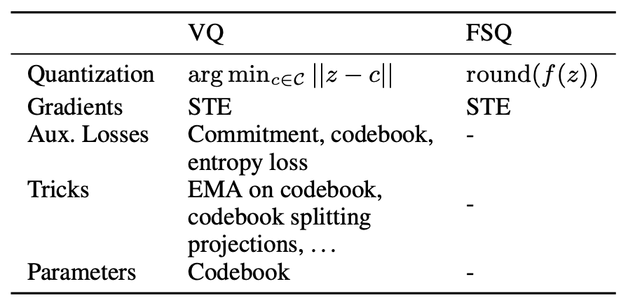 ] Comparison between VQ and FSQ (from the original paper)
Experiments
If we think of VQ as directly clustering encoding vectors into $K$ distinct categories, then FSQ instead summarizes the encoding vector into $d$ attributes, each divided into $L$ levels, thereby directly representing $L^d$ distinct integers. More generally, of course, the number of levels for each attribute can differ, denoted $L_1,L_2,\cdots,L_d$, giving a total number of combinations of $L_1 L_2\cdots L_d$.
Following the original paper's recommendation $L\geq 5$ (the earlier LFQ] is essentially equivalent to $L=2$), to match VQ-VAE's number of codes $K$, FSQ requires $d = \log_L K$—meaning FSQ imposes a restriction on the dimensionality $d$ of the encoding vector (generally kept to a single digit), which is usually far smaller than VQ-VAE's encoding dimension (typically three digits). A direct consequence of this is that when the total number of codes $K$ is relatively small (and hence $d$ is also small), FSQ tends to underperform relative to VQ:
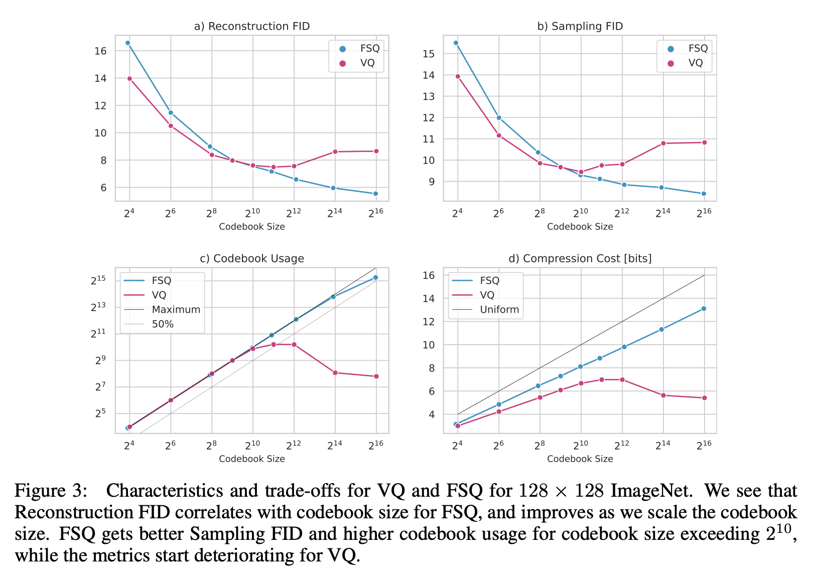 ] Difference in performance between VQ and FSQ at different codebook sizes
As the figure shows, when the codebook size is around 1000, FSQ and VQ perform similarly; when the codebook size significantly exceeds 1000, FSQ has the edge; conversely, when the codebook size is significantly smaller than 1000, VQ wins out. This matches my own experimental findings. My reference code is here:
GitHub: https://github.com/bojone/FSQ]
The remaining experiments are fairly standard demonstrations of FSQ outperforming VQ across various tasks—interested readers can consult the original paper directly.
Reflections
Formally speaking, if we assume $K=L^d$, then VQ is like "a classifier with $L^d$ classes," while FSQ is like "$d$ raters each scoring on a scale of $L$." Whether judged by parameter count, geometric intuition, or expressive power, FSQ is actually inferior to VQ. So why does FSQ have a chance of outperforming VQ? I think there are two reasons.
The first reason is that the encoder and decoder are simply too strong. Although FSQ itself is weaker, the encoder and decoder are powerful enough that, under the assumption of the universal approximation capability of neural networks, they can fully compensate for FSQ's disadvantage relative to VQ. Under the setting where $K=L^d$, the degree of discretization is the same for both methods—meaning the "information bottleneck" between encoder and decoder is identical—so the shortcomings of FSQ itself become negligible.
The second reason is that VQ's "teammate" (the gradient) is too weak. A classic problem with VQ is codebook collapse: as the codebook grows larger, it isn't fully utilized; instead, due to destructive competition, entries in the codebook cluster together. The classic symptom is a codebook of size 5000 ending up performing worse than one of size 500. Ultimately, this comes down to the gradient not being ideal enough. Even though VQ cleverly designs its gradient, for a hard-assignment operation like $\mathop{\text{argmin}}$, gradient-based optimization inevitably suffers from a "winner-takes-all" problem—this is the fundamental cause of collapse. FSQ's $\text{Round}$ operation, by contrast, involves no assignment at all; it simply takes a direct numerical approximation. Indeed, speaking more broadly, K-Means—which is similar in spirit to VQ—often suffers from cluster-center collapse as well, so it's clear that the difficulty of optimizing $\mathop{\text{argmin}}$ has long been a thorny problem. So rather than saying FSQ is especially strong, it's more accurate to say that VQ's "teammate" is especially weak.
From the above two points, we can see that for FSQ to surpass VQ, besides needing a sufficiently large codebook, it also needs a sufficiently complex encoder and decoder—but this isn't always guaranteed. For instance, in some scenarios we may want every layer's output in the model to be quantized, in which case the encoder and decoder capacity, once distributed across layers, may not be complex enough, and FSQ's inherent shortcomings then become the bottleneck on performance. Furthermore, the vector dimensionality after VQ doesn't change and can be arbitrarily high, whereas the vector before FSQ must be projected down to $d = \log_L K$ dimensions—a severe dimensionality reduction. When we need to recover a high-dimensional approximate vector from before the projection, it's very difficult to reconstruct it simply from the low-dimensional vector produced after FSQ.
So, if the goal is purely to serve as an "image tokenizer," FSQ may already be able to replace VQ—but that doesn't mean VQ can be replaced by FSQ in every scenario.
Summary
This article introduced an extremely simple substitute for the "VQ" in VQ-VAE—FSQ (Finite Scalar Quantization)—which discretizes continuous vectors directly through rounding, requiring no additional auxiliary loss. Experimental results show that when the codebook is large enough, FSQ has an advantage over VQ.
Translated automatically with claude-sonnet-5; all equations are reproduced verbatim from the source. Copyright remains with the original author.