Generative Diffusion Models: A Rambling Introduction (I): DDPM = Demolition + Construction
Among generative models, VAE] and GAN] are practically household names, and this blog has discussed them many times before. There are also some more niche choices, such as flow-based models] and VQ-VAE], which have quite a following too — especially VQ-VAE and its variant VQ-GAN], which has gradually risen to the status of an "image tokenizer," used to directly bring various NLP pretraining methods over to the image domain. Besides all of these, there is another choice that used to be even more niche — diffusion models — which is now taking the generative modeling world by storm. Two of the current state-of-the-art text-to-image models, OpenAI's DALL·E 2] and Google's Imagen], are both built on diffusion models.
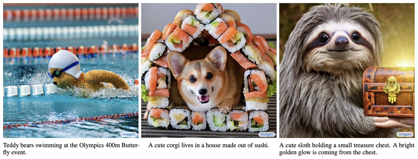 ] Some examples of Imagen "text-to-image" generation
Starting with this post, I'm opening up a new series to gradually cover the progress made over the past couple of years on generative diffusion models. Diffusion models are said to be famous for their mathematical complexity, apparently much harder to understand than VAEs or GANs — but is that really true? Is it really impossible to give an intuitive, "plain-language" understanding of diffusion models? Let's find out. more
A New Starting Point
Actually, we've briefly touched on diffusion models before, in GANs from an Energy Perspective (III): Generative Models = Energy Models] and From Denoising Autoencoders to Generative Models]. When people talk about diffusion models, they typically bring up energy-based models, score matching, the Langevin equation, and so on. In short, the idea is to train an energy-based model via techniques like score matching, and then use the Langevin equation to sample from that energy model.
In theory, this is a well-established framework that can, in principle, be used to generate and sample any continuous-valued object (speech, images, etc.). In practice, however, training an energy function is a genuinely hard problem, especially when the data dimensionality is large (e.g. high-resolution images) — it's very difficult to train a well-behaved energy function. On top of that, sampling from an energy model via the Langevin equation carries a lot of uncertainty, and the resulting samples are often noisy. For a long time, this traditional line of diffusion models was thus mostly confined to experiments on fairly low-resolution images.
The current explosion of interest in generative diffusion models actually began with DDPM] (Denoising Diffusion Probabilistic Model), proposed in 2020. Although it also uses the name "diffusion model," in fact — apart from a certain formal resemblance in the sampling procedure — DDPM is completely different from traditional Langevin-sampling-based diffusion models. It represents a genuinely new starting point, a new chapter altogether.
Strictly speaking, DDPM would more accurately be called a "gradual transformation model"; the name "diffusion model" is actually rather misleading. Concepts from traditional diffusion models — energy models, score matching, the Langevin equation — really have nothing to do with DDPM or its subsequent variants. Interestingly, the mathematical framework of DDPM had already been laid out in the ICML 2015 paper Deep Unsupervised Learning using Nonequilibrium Thermodynamics], but it was DDPM that first got this framework working for high-resolution image generation, which is what triggered the ensuing wave of enthusiasm. This shows that the birth and popularity of a model often also depend on timing and opportunity.
Demolition and Construction
Many articles, when introducing DDPM, jump straight into transition distributions, then variational inference, and a pile of notation — scaring off a good number of readers right off the bat (though, from this style of introduction, we can indeed see that DDPM is really a VAE rather than a diffusion model in the traditional sense). Combined with people's preconceptions about traditional diffusion models, this has created the illusion that DDPM "requires deep mathematical knowledge." In fact, DDPM can also be understood in a very plain, intuitive way — it's not any harder than GANs, which have that familiar "counterfeiter vs. detective" analogy.
First, suppose we want to build a generative model like a GAN, which is really a process that transforms random noise $\boldsymbol{z}$ into a data sample $\boldsymbol{x}$:
\begin{equation}\require{AMScd}\begin{CD} \text{random noise}\boldsymbol{z}\quad @>\quad\text{transform}\quad>> \quad\text{sample data}\boldsymbol{x}\\ @V \text{analogy} VV @VV \text{analogy} V\\ \text{brick tile cement}\quad @>\quad\text{construction}\quad>> \quad\text{skyscraper}\\ \end{CD}\end{equation}
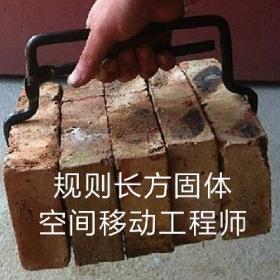 ] Please, call me an engineer
We can picture this process as "construction," where the random noise $\boldsymbol{z}$ is the raw material — bricks, cement, and so on — and the data sample $\boldsymbol{x}$ is the finished skyscraper. So a generative model is a construction crew that builds a skyscraper out of raw materials.
This process is certainly hard, which is why there's so much research on generative models. But as the saying goes, "destruction is easier than construction" — you may not know how to build a skyscraper, but surely you know how to demolish one? Let's consider the process of tearing down the skyscraper step by step into bricks and cement: let $\boldsymbol{x}_0$ be the finished skyscraper (the data sample), and $\boldsymbol{x}_T$ be the demolished bricks and cement (random noise). Suppose "demolition" takes $T$ steps; the whole process can be written as
\begin{equation}\boldsymbol{x} = \boldsymbol{x}_0 \to \boldsymbol{x}_1 \to \boldsymbol{x}_2 \to \cdots \to \boldsymbol{x}_{T-1} \to \boldsymbol{x}_T = \boldsymbol{z}\end{equation}
The difficulty in building the skyscraper lies in the fact that the gap between the raw material $\boldsymbol{x}_T$ and the finished skyscraper $\boldsymbol{x}_0$ is too large — an ordinary person can hardly grasp how $\boldsymbol{x}_T$ suddenly turns into $\boldsymbol{x}_0$. But once we have the intermediate "demolition" process $\boldsymbol{x}_1,\boldsymbol{x}_2,\cdots,\boldsymbol{x}_T$, we know that $\boldsymbol{x}_{t-1} \to \boldsymbol{x}_t$ represents one step of demolition — so isn't $\boldsymbol{x}_t\to \boldsymbol{x}_{t-1}$, run in reverse, exactly one step of construction? If we can learn the transformation relationship $\boldsymbol{x}_{t-1}=\boldsymbol{\mu}(\boldsymbol{x}_t)$ between the two, then starting from $\boldsymbol{x}_T$ and repeatedly applying $\boldsymbol{x}_{T-1}=\boldsymbol{\mu}(\boldsymbol{x}_T)$, $\boldsymbol{x}_{T-2}=\boldsymbol{\mu}(\boldsymbol{x}_{T-1})$, ..., won't we eventually end up building the skyscraper $\boldsymbol{x}_0$?
How to Demolish
As the saying goes, "you have to eat rice one mouthful at a time" — and buildings, too, have to be built one step at a time. The process by which DDPM builds a generative model is exactly the same as this "demolition-then-construction" analogy: it first works backwards, constructing a process that gradually transforms a data sample into random noise, and then considers the inverse transformation, generating data samples by repeatedly applying this inverse transformation. This is why I said earlier that DDPM should more accurately be called a "gradual transformation model" rather than a "diffusion model."
Specifically, DDPM models the "demolition" process as
\begin{equation}\boldsymbol{x}_t = \alpha_t \boldsymbol{x}_{t-1} + \beta_t \boldsymbol{\varepsilon}_t,\quad \boldsymbol{\varepsilon}_t\sim\mathcal{N}(\boldsymbol{0}, \boldsymbol{I})\label{eq:forward}\end{equation}
where $\alpha_t,\beta_t > 0$ and $\alpha_t^2 + \beta_t^2=1$ hold, and $\beta_t$ is usually very close to 0, representing the degree of damage done to the original structure in a single "demolition" step. The introduction of the noise $\boldsymbol{\varepsilon}_t$ represents a kind of corruption of the original signal — we can also think of it as "raw material": at every demolition step, we decompose $\boldsymbol{x}_{t-1}$ into "a $\alpha_t \boldsymbol{x}_{t-1}$ fraction of the building + a $\beta_t \boldsymbol{\varepsilon}_t$ fraction of raw material." (Note: the definition of $\alpha_t,\beta_t$ here differs from that in the original paper.)
Applying this demolition step repeatedly, we get:
\begin{equation}\begin{aligned} \boldsymbol{x}_t =&\, \alpha_t \boldsymbol{x}_{t-1} + \beta_t \boldsymbol{\varepsilon}_t \\ =&\, \alpha_t \big(\alpha_{t-1} \boldsymbol{x}_{t-2} + \beta_{t-1} \boldsymbol{\varepsilon}_{t-1}\big) + \beta_t \boldsymbol{\varepsilon}_t \\ =&\,\cdots\\ =&\,(\alpha_t\cdots\alpha_1) \boldsymbol{x}_0 + \underbrace{(\alpha_t\cdots\alpha_2)\beta_1 \boldsymbol{\varepsilon}_1 + (\alpha_t\cdots\alpha_3)\beta_2 \boldsymbol{\varepsilon}_2 + \cdots + \alpha_t\beta_{t-1} \boldsymbol{\varepsilon}_{t-1} + \beta_t \boldsymbol{\varepsilon}_t}_{\text{sum of independent normal noises}} \end{aligned}\label{eq:expand}\end{equation}
At this point, readers might be wondering why the accumulated coefficients need to satisfy $\alpha_t^2 + \beta_t^2 = 1$ — now we can answer that question. First, the part marked with braces in the equation is exactly the sum of several independent normal noise terms, with mean 0 and variances $(\alpha_t\cdots\alpha_2)^2\beta_1^2$, $(\alpha_t\cdots\alpha_3)^2\beta_2^2$, ..., $\alpha_t^2\beta_{t-1}^2$, $\beta_t^2$ respectively; next, we use a fact from probability theory — the additivity of normal distributions — namely that the sum of these independent normal noise terms is itself normally distributed, with mean 0 and variance $(\alpha_t\cdots\alpha_2)^2\beta_1^2 + (\alpha_t\cdots\alpha_3)^2\beta_2^2 + \cdots + \alpha_t^2\beta_{t-1}^2 + \beta_t^2$; finally, under the constraint that $\alpha_t^2 + \beta_t^2 = 1$ always holds, we find that the sum of squares of the coefficients in equation $\eqref{eq:expand}$ is still 1, i.e.
\begin{equation}(\alpha_t\cdots\alpha_1)^2 + (\alpha_t\cdots\alpha_2)^2\beta_1^2 + (\alpha_t\cdots\alpha_3)^2\beta_2^2 + \cdots + \alpha_t^2\beta_{t-1}^2 + \beta_t^2 = 1\end{equation}
so in fact we effectively have
\begin{equation}\boldsymbol{x}_t = \underbrace{(\alpha_t\cdots\alpha_1)}_{\text{denote}\bar{\alpha}_t} \boldsymbol{x}_0 + \underbrace{\sqrt{1 - (\alpha_t\cdots\alpha_1)^2}}_{\text{denote}\bar{\beta}_t} \bar{\boldsymbol{\varepsilon}}_t,\quad \bar{\boldsymbol{\varepsilon}}_t\sim\mathcal{N}(\boldsymbol{0}, \boldsymbol{I})\label{eq:skip}\end{equation}
This gives us a great deal of convenience when computing $\boldsymbol{x}_t$. On another note, DDPM chooses an appropriate form for $\alpha_t$ such that $\bar{\alpha}_T\approx 0$ holds, meaning that after $T$ steps of demolition, essentially nothing of the original building remains — it has all been converted into raw material $\boldsymbol{\varepsilon}$. (Note: the definition of $\bar{\alpha}_t$ here again differs from that in the original paper.)
And How to Build
"Demolition" is the process of $\boldsymbol{x}_{t-1}\to \boldsymbol{x}_t$, and from this process we obtain a large number of data pairs $(\boldsymbol{x}_{t-1},\boldsymbol{x}_t)$. "Construction," naturally, then means learning a model of $\boldsymbol{x}_t\to \boldsymbol{x}_{t-1}$ from these data pairs. Let this model be $\boldsymbol{\mu}(\boldsymbol{x}_t)$; the obvious learning scheme is then to minimize the Euclidean distance between the two:
\begin{equation}\left\Vert\boldsymbol{x}_{t-1} - \boldsymbol{\mu}(\boldsymbol{x}_t)\right\Vert^2\label{eq:loss-0}\end{equation}
This is already very close to the final DDPM model — let's now refine this a bit further. First, the "demolition" equation $\eqref{eq:forward}$ can be rewritten as $\boldsymbol{x}_{t-1} = \frac{1}{\alpha_t}\left(\boldsymbol{x}_t - \beta_t \boldsymbol{\varepsilon}_t\right)$, which suggests that we might design the "construction" model $\boldsymbol{\mu}(\boldsymbol{x}_t)$ to take the form
\begin{equation}\boldsymbol{\mu}(\boldsymbol{x}_t) = \frac{1}{\alpha_t}\left(\boldsymbol{x}_t - \beta_t \boldsymbol{\epsilon}_{\boldsymbol{\theta}}(\boldsymbol{x}_t, t)\right)\label{eq:sample}\end{equation}
where $\boldsymbol{\theta}$ is a trainable parameter. Substituting this into the loss function gives
\begin{equation}\left\Vert\boldsymbol{x}_{t-1} - \boldsymbol{\mu}(\boldsymbol{x}_t)\right\Vert^2 = \frac{\beta_t^2}{\alpha_t^2}\left\Vert \boldsymbol{\varepsilon}_t - \boldsymbol{\epsilon}_{\boldsymbol{\theta}}(\boldsymbol{x}_t, t)\right\Vert^2\end{equation}
The factor $\frac{\beta_t^2}{\alpha_t^2}$ out front represents a loss weight, which we can ignore for now. Finally, substituting the expression for $\boldsymbol{x}_t$ given by combining equations $\eqref{eq:skip}$ and $\eqref{eq:forward}$,
\begin{equation}\boldsymbol{x}_t = \alpha_t\boldsymbol{x}_{t-1} + \beta_t \boldsymbol{\varepsilon}_t = \alpha_t\left(\bar{\alpha}_{t-1}\boldsymbol{x}_0 + \bar{\beta}_{t-1}\bar{\boldsymbol{\varepsilon}}_{t-1}\right) + \beta_t \boldsymbol{\varepsilon}_t = \bar{\alpha}_t\boldsymbol{x}_0 + \alpha_t\bar{\beta}_{t-1}\bar{\boldsymbol{\varepsilon}}_{t-1} + \beta_t \boldsymbol{\varepsilon}_t \end{equation}
we obtain the loss function in the form
\begin{equation}\left\Vert \boldsymbol{\varepsilon}_t - \boldsymbol{\epsilon}_{\boldsymbol{\theta}}(\bar{\alpha}_t\boldsymbol{x}_0 + \alpha_t\bar{\beta}_{t-1}\bar{\boldsymbol{\varepsilon}}_{t-1} + \beta_t \boldsymbol{\varepsilon}_t, t)\right\Vert^2\label{eq:loss-1}\end{equation}
Readers might wonder why we back up one step to express $\boldsymbol{x}_t$ this way — can't we just directly give $\boldsymbol{x}_t$ based on equation $\eqref{eq:skip}$? The answer is no, because we have already sampled $\boldsymbol{\varepsilon}_t$ ahead of time, and $\boldsymbol{\varepsilon}_t$ is not independent of $\bar{\boldsymbol{\varepsilon}}_t$; so given $\boldsymbol{\varepsilon}_t$, we can't sample $\bar{\boldsymbol{\varepsilon}}_t$ completely independently.
Reducing the Variance
In principle, the loss function $\eqref{eq:loss-1}$ is already enough to train DDPM. But in practice it runs the risk of having too high a variance, which can lead to slow convergence and other issues. It's easy to see why: equation $\eqref{eq:loss-1}$ actually involves 4 random variables that need to be sampled:
1. Sample one $\boldsymbol{x}_0$ from all the training samples;
2. Sample $\bar{\boldsymbol{\varepsilon}}_{t-1}, \boldsymbol{\varepsilon}_t$ from the normal distribution $\mathcal{N}(\boldsymbol{0}, \boldsymbol{I})$ (two separate sampling outcomes);
3. Sample one $t$ from $1\sim T$.
The more random variables that need to be sampled, the harder it is to get an accurate estimate of the loss function — in other words, each estimate of the loss will fluctuate (have variance) more heavily. Fortunately, we can use an integration trick to merge $\bar{\boldsymbol{\varepsilon}}_{t-1}, \boldsymbol{\varepsilon}_t$ into a single normal random variable, which alleviates the high-variance problem somewhat.
This integral does involve a bit of a trick, but it's not too complicated. Thanks to the additivity of normal distributions, we know that $\alpha_t\bar{\beta}_{t-1}\bar{\boldsymbol{\varepsilon}}_{t-1} + \beta_t \boldsymbol{\varepsilon}_t$ is effectively equivalent to a single random variable $\bar{\beta}_t\boldsymbol{\varepsilon}|\boldsymbol{\varepsilon}\sim \mathcal{N}(\boldsymbol{0}, \boldsymbol{I})$; likewise, $\beta_t \bar{\boldsymbol{\varepsilon}}_{t-1} - \alpha_t\bar{\beta}_{t-1} \boldsymbol{\varepsilon}_t$ is effectively equivalent to a single random variable $\bar{\beta}_t\boldsymbol{\omega}|\boldsymbol{\omega}\sim \mathcal{N}(\boldsymbol{0}, \boldsymbol{I})$, and one can verify that $\mathbb{E}[\boldsymbol{\varepsilon}\boldsymbol{\omega}^{\top}]=\boldsymbol{0}$ holds, so these are two mutually independent normal random variables.
Next, we go the other way and re-express $\boldsymbol{\varepsilon}_t$ in terms of $\boldsymbol{\varepsilon},\boldsymbol{\omega}$:
\begin{equation}\boldsymbol{\varepsilon}_t = \frac{(\beta_t \boldsymbol{\varepsilon} - \alpha_t\bar{\beta}_{t-1} \boldsymbol{\omega})\bar{\beta}_t}{\beta_t^2 + \alpha_t^2\bar{\beta}_{t-1}^2} = \frac{\beta_t \boldsymbol{\varepsilon} - \alpha_t\bar{\beta}_{t-1} \boldsymbol{\omega}}{\bar{\beta}_t}\end{equation}
Substituting this into equation $\eqref{eq:loss-1}$ gives
\begin{equation}\begin{aligned} &\,\mathbb{E}_{\bar{\boldsymbol{\varepsilon}}_{t-1}, \boldsymbol{\varepsilon}_t\sim \mathcal{N}(\boldsymbol{0}, \boldsymbol{I})}\left[\left\Vert \boldsymbol{\varepsilon}_t - \boldsymbol{\epsilon}_{\boldsymbol{\theta}}(\bar{\alpha}_t\boldsymbol{x}_0 + \alpha_t\bar{\beta}_{t-1}\bar{\boldsymbol{\varepsilon}}_{t-1} + \beta_t \boldsymbol{\varepsilon}_t, t)\right\Vert^2\right] \\ =&\,\mathbb{E}_{\boldsymbol{\omega}, \boldsymbol{\varepsilon}\sim \mathcal{N}(\boldsymbol{0}, \boldsymbol{I})}\left[\left\Vert \frac{\beta_t \boldsymbol{\varepsilon} - \alpha_t\bar{\beta}_{t-1} \boldsymbol{\omega}}{\bar{\beta}_t} - \boldsymbol{\epsilon}_{\boldsymbol{\theta}}(\bar{\alpha}_t\boldsymbol{x}_0 + \bar{\beta}_t\boldsymbol{\varepsilon}, t)\right\Vert^2\right] \end{aligned}\end{equation}
Notice that the loss function is now only quadratic in $\boldsymbol{\omega}$, so we can expand it and compute its expectation directly, obtaining
\begin{equation}\frac{\beta_t^2}{\bar{\beta}_t^2}\mathbb{E}_{\boldsymbol{\varepsilon}\sim \mathcal{N}(\boldsymbol{0}, \boldsymbol{I})}\left[\left\Vert\boldsymbol{\varepsilon} - \frac{\bar{\beta}_t}{\beta_t}\boldsymbol{\epsilon}_{\boldsymbol{\theta}}(\bar{\alpha}_t\boldsymbol{x}_0 + \bar{\beta}_t\boldsymbol{\varepsilon}, t)\right\Vert^2\right]+\text{const}\end{equation}
Once again dropping the constant term and the loss weight, we arrive at the loss function ultimately used by DDPM:
\begin{equation}\left\Vert\boldsymbol{\varepsilon} - \frac{\bar{\beta}_t}{\beta_t}\boldsymbol{\epsilon}_{\boldsymbol{\theta}}(\bar{\alpha}_t\boldsymbol{x}_0 + \bar{\beta}_t\boldsymbol{\varepsilon}, t)\right\Vert^2\end{equation}
(Note: the $\boldsymbol{\epsilon}_{\boldsymbol{\theta}}$ in the original paper is in fact exactly the $\frac{\bar{\beta}_t}{\beta_t}\boldsymbol{\epsilon}_{\boldsymbol{\theta}}$ used here, so the results are entirely equivalent.)
Recursive Generation
At this point, we've worked our way through the entire DDPM training pipeline. That was quite a bit of material — I certainly wouldn't call it "easy" — but there's really nothing in it that's extraordinarily difficult either: we never needed the traditional machinery of energy functions or score matching, and we didn't even need variational inference. Just by drawing on the "demolition-construction" analogy and some basic probability theory, we arrive at exactly the same results as the original derivation. So this new wave of generative diffusion models, epitomized by DDPM, is not nearly as complicated as many readers imagine — you could say it's really a vivid way of modeling learning through a "decompose-and-recombine" process.
Once training is done, we can generate a sample starting from random noise $\boldsymbol{x}_T\sim\mathcal{N}(\boldsymbol{0}, \boldsymbol{I})$ by running equation $\eqref{eq:sample}$ for $T$ steps:
\begin{equation}\boldsymbol{x}_{t-1} = \frac{1}{\alpha_t}\left(\boldsymbol{x}_t - \beta_t \boldsymbol{\epsilon}_{\boldsymbol{\theta}}(\boldsymbol{x}_t, t)\right)\end{equation}
This corresponds to greedy search in autoregressive decoding. If we want random sampling instead, we need to add back in a noise term:
\begin{equation}\boldsymbol{x}_{t-1} = \frac{1}{\alpha_t}\left(\boldsymbol{x}_t - \beta_t \boldsymbol{\epsilon}_{\boldsymbol{\theta}}(\boldsymbol{x}_t, t)\right) + \sigma_t \boldsymbol{z},\quad \boldsymbol{z}\sim\mathcal{N}(\boldsymbol{0}, \boldsymbol{I})\end{equation}
Generally, we can set $\sigma_t=\beta_t$ so that the forward and backward variances stay in sync. This sampling process differs from Langevin sampling in traditional diffusion models in the following way: DDPM's sampling always starts from a fresh random noise sample, and must iterate $T$ times to produce one output sample; Langevin sampling, on the other hand, starts from an arbitrary point and iterates indefinitely — in theory, over the course of infinitely many iterations, every possible data sample gets generated at some point. So although the two look formally similar, they are, at heart, two fundamentally different models.
Looking at this generation process, we can sense that it's really the same as the decoding process in Seq2Seq — both are chained, autoregressive generation — so generation speed is a bottleneck. DDPM sets $T=1000$, meaning that generating a single image requires running $\boldsymbol{\epsilon}_{\boldsymbol{\theta}}(\boldsymbol{x}_t, t)$ 1000 times. This is a major drawback of DDPM: slow sampling speed, and much subsequent work has focused on speeding up DDPM sampling. Speaking of "image generation + autoregressive model + very slow," some readers might think of earlier models like PixelRNN] and PixelCNN], which turned image generation into a language modeling task, and were therefore likewise slow due to recursive sampling. So what's the real difference between DDPM's autoregressive generation and that of PixelRNN/PixelCNN? Why didn't PixelRNN/PixelCNN take off the way DDPM has?
Readers familiar with PixelRNN/PixelCNN know that these models generate images pixel by pixel, and autoregressive generation is inherently ordered — meaning we have to decide, ahead of time, an ordering over the pixels of the image, and the final generation quality is closely tied to this ordering. However, right now this ordering can only be designed by hand, based on experience (this kind of hand-designed prior knowledge is collectively called "inductive bias"), and there's currently no known theoretically optimal solution. In other words, PixelRNN/PixelCNN's generation quality is heavily influenced by inductive bias. DDPM is different: it defines a new "autoregressive direction" via the "demolition" process, one under which all pixels are treated equally and without bias, thereby reducing the influence of inductive bias and improving generation quality. Moreover, the number of iteration steps in DDPM generation is fixed $T$, whereas for PixelRNN/PixelCNN it equals the image resolution ($\text{width}\times\text{high}\times{通道数}$), so DDPM is much faster than PixelRNN/PixelCNN when generating high-resolution images.
Hyperparameter Settings
In this section, let's discuss the setting of hyperparameters.
In DDPM, $T=1000$ — which may be a larger number than many readers expect. So why choose such a large $T$? Also, as for the choice of $\alpha_t$, translating the original paper's settings into this blog's notation gives roughly
\begin{equation}\alpha_t = \sqrt{1 - \frac{0.02t}{T}}\end{equation}
This is a monotonically decreasing function — so why choose a monotonically decreasing $\alpha_t$?
These two questions actually have closely related answers, tied to the specifics of the data domain. For simplicity, when reconstructing, we used the Euclidean distance $\eqref{eq:loss-0}$ as the loss function. Generally, when we use DDPM for image generation, anyone who's worked on image generation before knows that Euclidean distance isn't a good measure of how "realistic" an image looks. When VAEs use Euclidean distance for reconstruction, they tend to produce blurry results, and it's only when the input and output images are very close to each other that Euclidean distance gives reasonably sharp results. So choosing as large a $T$ as possible is precisely meant to keep the input and output as close as possible, reducing the blurriness caused by the Euclidean-distance loss.
The choice of a monotonically decreasing $\alpha_t$ follows similar reasoning. When $t$ is small, $\boldsymbol{x}_t$ is still fairly close to the real image, so we want to keep $\boldsymbol{x}_{t-1}$ and $\boldsymbol{x}_t$ close together, so that the Euclidean distance $\eqref{eq:loss-0}$ is more appropriate — hence we need a larger $\alpha_t$. When $t$ is large, $\boldsymbol{x}_t$ is already close to pure noise, and using Euclidean distance for noise is not a problem, so we can afford to widen the gap between $\boldsymbol{x}_{t-1}$ and $\boldsymbol{x}_t$ somewhat — i.e., use a smaller $\alpha_t$. So could we just use a large $\alpha_t$ throughout? We could, but we'd need to increase $T$. Recall that when deriving $\eqref{eq:skip}$, we noted that we should have $\bar{\alpha}_T\approx 0$, and we can estimate this directly:
\begin{equation}\log \bar{\alpha}_T = \sum_{t=1}^T \log\alpha_t = \frac{1}{2} \sum_{t=1}^T \log\left(1 - \frac{0.02t}{T}\right) < \frac{1}{2} \sum_{t=1}^T \left(- \frac{0.02t}{T}\right) = -0.005(T+1)\end{equation}
Substituting in $T=1000$ gives roughly $\bar{\alpha}_T\approx e^{-5}$, which happens to just about meet the $\approx 0$ criterion. So if we used a large $\alpha_t$ throughout, we would necessarily need a much larger $T$ in order for $\bar{\alpha}_T\approx 0$ to hold.
Finally, notice that in the "construction" model $\boldsymbol{\epsilon}_{\boldsymbol{\theta}}(\bar{\alpha}_t\boldsymbol{x}_0 + \bar{\beta}_t\boldsymbol{\varepsilon}, t)$, we explicitly include $t$ as an input. This is because, in principle, different values of $t$ correspond to different levels of the object, and so should really be handled by different reconstruction models — that is, we should in principle have $T$ distinct reconstruction models. Instead, we share the parameters across all of these reconstruction models, and pass in $t$ as a conditioning signal. According to the paper's appendix, $t$ is converted into the positional encoding described in The Path to Transformer Upgrades: 1. Tracing the Origins of Sinusoidal Positional Encoding] and then added directly onto the residual blocks.
Summary
This post introduced the latest generative diffusion model, DDPM, through the intuitive analogy of "demolition and construction." From this perspective, we've been able to arrive at results that are identical to those in the original paper using fairly plain language and comparatively little mathematical derivation. In short, this post has shown that DDPM, too, can be given a vivid analogy just like GANs — it needs neither the "variational" machinery of VAEs, nor the "probability divergence" or "optimal transport" concepts of GANs. In this sense, DDPM could even be considered simpler than either VAEs or GANs.
Translated automatically with claude-sonnet-5; all equations are reproduced verbatim from the source. Copyright remains with the original author.