A Concise Introduction to VQ-VAE: Quantized Autoencoders
As I recall, I came across VQ-VAE a long time ago, and back then I didn't have much interest in it. Recently, though, two things rekindled my interest. First, VQ-VAE-2 achieved generation quality that can match BigGAN's (as reported by Synced); second, while recently reading an NLP paper, Unsupervised Paraphrasing without Translation, I found that it also uses VQ-VAE. These two things suggest that VQ-VAE must be a fairly general and interesting model, so I decided to dig into it properly.
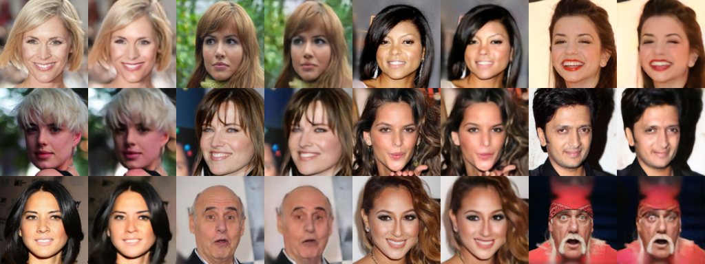 Reconstruction results of my own reproduction of VQ-VAE on CelebA. Note that details are preserved reasonably well, but a slight blurriness becomes noticeable when you zoom in.more
Overview of the model
VQ-VAE (Vector Quantised - Variational AutoEncoder) first appeared in the paper Neural Discrete Representation Learning, and just like VQ-VAE-2, it's another impressive work from a Google team.
Interesting, yet somewhat mystifying
As an autoencoder, one obvious characteristic of VQ-VAE is that the encoding vector it produces is discrete. In other words, every element of the final encoding vector is an integer — this is exactly what "Quantised" refers to. We might call this "quantization" (in the same sense as "quantum" in quantum mechanics, which also implies discretization).
Given that the entire model is continuous and differentiable, yet the resulting encoding vector ends up discrete, and the reconstructions still look quite sharp (as in the image at the top of this post), this at least suggests that VQ-VAE must contain some interesting and valuable tricks worth learning. However, after reading the original paper, I couldn't shake the feeling that it was written in a somewhat hard-to-follow way. This isn't the kind of difficulty you get from a paper like the original ON-LSTM paper, which is genuinely dense and technical — it's more a feeling of unnecessary mystification.
First, once you finish reading the whole paper, you realize that VQ-VAE is actually just an AE (autoencoder), not a VAE (variational autoencoder). I don't know what motivated the authors to insist on using probabilistic language to associate it with VAEs, but this clearly makes the paper harder to understand than it needs to be. Second, one of the core steps of VQ-VAE is the Straight-Through Estimator, a trick for optimizing through discretized latent variables, and the original paper doesn't explain it in any real detail — you basically have to read the source code to understand what's going on. Finally, the core idea of the paper isn't well laid out either; it feels like the paper is purely describing the model itself without explaining the thinking behind it.
PixelCNN
To trace the origins of VQ-VAE's ideas, we need to talk about autoregressive models. It's fair to say that VQ-VAE's approach to generative modeling stems from autoregressive models like PixelRNN and PixelCNN. These models observe that the images we want to generate are actually discrete rather than continuous. Take a CIFAR-10 image as an example: it's a 3-channel image of size $32\times 32$, in other words a $32\times 32\times 3$ matrix, where each element of the matrix is some integer between 0 and 255. We can therefore think of it as a "sentence" of length $32\times 32\times 3=3072$, with a vocabulary size of 256, and use language-model-style methods to generate the image pixel by pixel, recursively (conditioning on all the preceding pixels to predict the next one). This is the so-called autoregressive approach:
\begin{equation}p(x)=p(x_1)p(x_2|x_1)\dots p(x_{3n^2}|x_1,x_2,\dots,x_{3n^2-1})\end{equation}
where each of the $p(x_1),p(x_2|x_1),\dots,p(x_{3n^2}|x_1,x_2,\dots,x_{3n^2-1})$ terms is a 256-way classification problem, differing only in what condition it depends on.
There's already plenty of material online about PixelRNN and PixelCNN, so I won't go over the details here — though I do feel one could ride the wave of Bert's popularity and cook up a "PixelAtt" (Attention) variant. Research on autoregressive models mainly focuses on two things: one is how to design the recursive ordering so that the model can generate/sample better, since an image's sequence isn't a simple 1D sequence — it's at least 2D, and often 3D — and whether you go "left to right, then top to bottom," "top to bottom then left to right," "center first then outward," or some other order, this has a big effect on generation quality; the other direction is how to speed up the sampling process. Among the papers I've read, a relatively recent achievement in autoregressive modeling is the ICLR 2019 work Generating High Fidelity Images with Subscale Pixel Networks and Multidimensional Upscaling.
The autoregressive approach is reliable and can effectively estimate probabilities, but it has one fatal drawback: it's slow. Because generation proceeds pixel by pixel, each pixel needs to be sampled individually. The CIFAR-10 example above is already a small image; nowadays, to be taken seriously for image generation you really need to be working at resolutions around $128\times 128\times 3$, which comes to nearly 50,000 pixels in total (imagine generating a "sentence" of length 50,000) — generating pixel by pixel at that scale would be extremely time-consuming. And with such a long sequence, neither RNNs nor CNNs can capture such long-range dependencies well.
There's another problem with the vanilla autoregressive approach: it severs the connections between adjacent categories. Since each pixel is discrete, treating it as a 256-way classification problem is fine in principle, but in reality, the difference between adjacent pixel values is tiny, and a pure classification objective fails to capture this relationship. Put more mathematically: our cross-entropy objective is $-\log p_t$. Suppose the target pixel value is 100, and I predict 99 — because these are different classes, $p_t$ will be close to 0 and $-\log p_t$ will be large, incurring a large loss. But visually speaking, there's barely any difference between a pixel value of 100 and 99, so it shouldn't incur such a large penalty.
VQ-VAE
To address these inherent flaws of autoregressive models, VQ-VAE's proposed solution is: first reduce the dimensionality, then model the resulting encoding vectors with PixelCNN.
Dimensionality reduction plus discretization
This sounds like a natural plan at first glance, nothing special — but it's actually far from natural.
The reason is that since PixelCNN generates discrete sequences, if you want to model the encoding vectors with PixelCNN, those encoding vectors also need to be discrete. But our usual dimensionality-reduction tools, such as autoencoders, produce continuous-valued encoding vectors and cannot directly produce discrete variables. Moreover, generating discrete variables usually comes with the problem of vanishing gradients. And on top of that, in this whole process of reducing dimensionality and then reconstructing, how do we ensure the reconstructed image isn't badly distorted? If the distortion is too severe — worse even than an ordinary VAE — then VQ-VAE would have no reason to exist.
Fortunately, VQ-VAE does provide an effective training strategy that solves both problems.
Nearest-neighbor reconstruction
In VQ-VAE, an image $x$ of size $n\times n\times 3$ is first fed into a $encoder$, producing a continuous encoding vector $z$:
\begin{equation}z = encoder(x)\end{equation}
Here $z$ is a vector of size $d$. In addition, VQ-VAE maintains an embedding layer, which we can also call the codebook, denoted as
\begin{equation}E = [e_1, e_2, \dots, e_K]\end{equation}
where each $e_i$ is a vector of size $d$. Next, VQ-VAE uses a nearest-neighbor search to map $z$ to one of these $K$ vectors:
\begin{equation}z\to e_k,\quad k = \mathop{\text{argmin}}_j \Vert z - e_j\Vert_2\end{equation}
We denote the codebook vector corresponding to $z$ as $z_q$, and we treat $z_q$ as the final encoding result. Finally, $z_q$ is passed into a $decoder$, with the goal of reconstructing the original image $\hat{x}=decoder(z_q)$.
The overall pipeline is:
\begin{equation}x\xrightarrow{encoder} z \xrightarrow{\text{nearest neighbor}} z_q \xrightarrow{decoder}\hat{x}\end{equation}
Since $z_q$ is one of the vectors in the codebook $E$, it is effectively equivalent to one of the $1,2,\dots,K$ integers among $K$, so this whole pipeline is equivalent to encoding the entire image as a single integer.
Of course, the above process is simplified. If we only encode the image into a single vector, reconstruction quality will inevitably suffer, and it will be hard to guarantee good generalization. So in practice, we use several convolutional layers to encode $x$ directly into $m\times m$ vectors, each of size $d$:
\begin{equation}z = \begin{pmatrix}z_{11} & z_{12} & \dots & z_{1m}\\ z_{21} & z_{22} & \dots & z_{2m}\\ \vdots & \vdots & \ddots & \vdots\\ z_{m1} & z_{m2} & \dots & z_{mm}\\ \end{pmatrix}\end{equation}
That is, the total size of $z$ is $m\times m\times d$, and it still retains spatial structure. Then, each vector is mapped to one entry in the codebook using the method described above, giving us an equally-sized $z_q$, which is then used for reconstruction. In this way, $z_q$ is also equivalent to an integer matrix of size $m\times m$, achieving discrete encoding.
Custom-designed gradients
As we know, for an ordinary autoencoder, we would simply train with the following loss:
\begin{equation}\Vert x - decoder(z)\Vert_2^2\end{equation}
But in VQ-VAE, what we actually use for reconstruction is $z_q$, not $z$, so it would seem we should use this loss instead:
\begin{equation}\Vert x - decoder(z_q)\Vert_2^2\end{equation}
The problem is that the construction of $z_q$ involves $\text{argmin}$, an operation with no gradient, so if we used the second loss, we would have no way of updating $encoder$.
In other words, our real objective is to minimize $\Vert x - decoder(z_q)\Vert_2^2$, but this isn't easy to optimize, whereas $\Vert x - decoder(z)\Vert_2^2$ is easy to optimize but isn't actually our objective. So what do we do? A rather crude approach, of course, would be to use both:
\begin{equation}\Vert x - decoder(z)\Vert_2^2 + \Vert x - decoder(z_q)\Vert_2^2\end{equation}
But this isn't ideal, because minimizing $\Vert x - decoder(z)\Vert_2^2$ isn't actually our goal — it introduces an extraneous constraint.
VQ-VAE uses an elegant and direct method called the Straight-Through Estimator (you could also call it "direct pass-through estimation"), which originates from Bengio's paper Estimating or Propagating Gradients Through Stochastic Neurons for Conditional Computation. Even in the original VQ-VAE paper, the authors simply cite this paper without offering much explanation. In fact, reading this original paper directly isn't a very friendly experience — you're better off just reading the source code.
The idea behind Straight-Through is actually simple: during the forward pass, you can use whatever variable you want (even if it's non-differentiable), and during the backward pass, you substitute in a gradient that you've designed yourself. Following this idea, the objective function we design is:
\begin{equation}\Vert x - decoder(z + sg[z_q - z])\Vert_2^2\end{equation}
where $sg$ denotes "stop gradient," meaning we discard its gradient. This way, during the forward pass (computing the loss), the expression is exactly equivalent to $decoder(z + z_q - z)=decoder(z_q)$; but during the backward pass (computing gradients), since $z_q - z$ contributes no gradient, it is equivalent to $decoder(z)$, which is what allows us to optimize $encoder$.
Incidentally, based on this same idea, we can define custom gradients for many functions ourselves. For instance, $x + sg[\text{relu}(x) - x]$ defines the gradient of $\text{relu}(x)$ to always be 1, while during loss computation it remains equivalent to $\text{relu}(x)$ itself. Of course, using the same trick, we can assign an arbitrary gradient to any function we like — whether that has any practical value depends entirely on the specific task at hand.
Maintaining the codebook
It's worth noting that, given how nearest-neighbor search is designed in VQ-VAE, we would expect $z_q$ and $z$ to be quite close to each other (in effect, each vector in the codebook $E$ acts like a cluster center for the corresponding $z$ vectors), but this isn't necessarily the case in practice. Even if both $\Vert x - decoder(z)\Vert_2^2$ and $\Vert x - decoder(z_q)\Vert_2^2$ are small individually, that doesn't mean $z_q$ and $z$ are close to each other (i.e., $f(z_1)=f(z_2)$ doesn't imply $z_1 = z_2$).
So, to make $z_q$ and $z$ closer, we can directly add $\Vert z - z_q\Vert_2^2$ to the loss:
\begin{equation}\Vert x - decoder(z + sg[z_q - z])\Vert_2^2 + \beta \Vert z - z_q\Vert_2^2\end{equation}
Beyond this, we can be even more careful. Since the codebook ($z_q$) is relatively free to move, while $z$ needs to focus on preserving reconstruction quality, we should generally prefer "moving $z_q$ towards $z$" over "moving $z$ towards $z_q$." And since the gradient of $\Vert z_q - z\Vert_2^2$ decomposes into the gradient with respect to $z_q$ plus the gradient with respect to $z$, we can equivalently split it as:
\begin{equation}\Vert sg[z] - z_q\Vert_2^2 + \Vert z - sg[z_q]\Vert_2^2\end{equation}
The first term corresponds to fixing $z$ and moving $z_q$ towards $z$, while the second term does the reverse — fixing $z_q$ and moving $z$ towards $z_q$. Note that this "equivalence" is with respect to the backward pass (gradient computation); for the forward pass (loss computation) it comes out to twice the original value. Given the reasoning above, since we want "moving $z_q$ towards $z$" to dominate over "moving $z$ towards $z_q$," we can adjust the relative weighting in the final loss:
\begin{equation}\Vert x - decoder(z + sg[z_q - z])\Vert_2^2 + \beta \Vert sg[z] - z_q\Vert_2^2 + \gamma \Vert z - sg[z_q]\Vert_2^2\end{equation}
where $\gamma < \beta$; the original paper uses $\gamma = 0.25 \beta$.
(Note: the codebook can also be updated via an exponential moving average — see the original paper for details.)
Fitting the distribution of the codes
After all this careful design, we've finally managed to encode an image into an integer matrix of size $m\times m$. Since this $m\times m$ matrix still retains, to some extent, the spatial structure of the original input image, we can use an autoregressive model such as PixelCNN to fit this code matrix (i.e., model its prior distribution). Once we obtain the distribution over codes via PixelCNN, we can randomly sample a new code matrix, map it through the codebook $E$ into a 3D real-valued tensor $z_q$ (rows × columns × encoding dimension), and finally pass it through $deocder$ to obtain an image.
Generally speaking, $m\times m$ is now much smaller than the original $n\times n\times 3$. For example, in my own experiments with the CelebA dataset, an original image of size $128\times 128\times 3$ could be encoded into a $32\times 32$ code with essentially no loss in quality. This means modeling the code matrix with an autoregressive model is much easier than modeling the raw image directly.
My own reproduction
Here is my own Keras implementation of VQ-VAE (Python 2.7 + Tensorflow 1.8 + Keras 2.2.4, with the model architecture partly based on this):
https://github.com/bojone/vae/blob/master/vq_vae_keras.py
The main body of this script only covers the encoding and reconstruction part of VQ-VAE (the image at the top of this post is a reconstruction produced with this script — as you can see, the reconstruction quality is decent), and does not include modeling the prior distribution with PixelCNN. However, the comments at the end of the script include an example using Attention to model the prior distribution. Here's what random sampling looks like after modeling the prior with Attention:
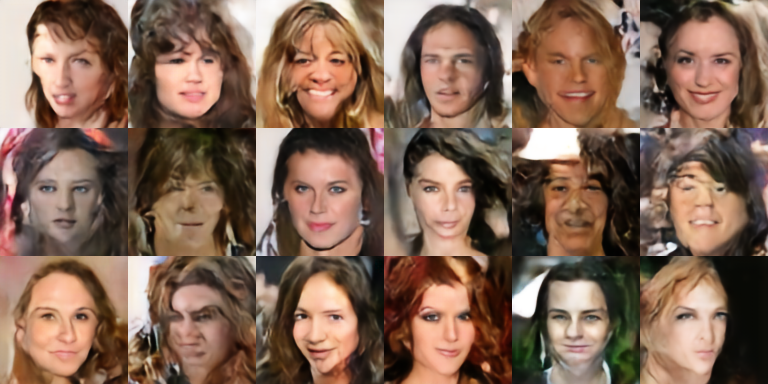 Random samples generated after modeling the prior distribution with my own PixelAtt (randomly selected, not cherry-picked)
These results show, to some extent, that this kind of random sampling is feasible, though the generation quality here isn't exactly great. I used PixelAtt rather than PixelCNN because, in my own reproduction, PixelCNN performed much worse than PixelAtt, so PixelAtt has a certain advantage — but its downside is that it's very GPU-memory hungry and prone to OOM errors. That said, the fact that my own reproduction isn't great doesn't mean the method itself is bad — it's quite possible I just didn't tune it well enough, or the network wasn't deep enough, and so on. Personally, I'm fairly bullish on this line of research into discrete encodings.
Final summary
At this point, I think I've explained VQ-VAE in a way I find reasonably clear. Looking back at the whole thing, there's really no trace of "VAE" flavor in it at all — which is why I say it's really just an AE, one that encodes into discrete vectors. The reason it can reconstruct fairly sharp images is that it retains a sufficiently large feature map during encoding.
Once you understand VQ-VAE, its newer version, 2.0, becomes easy to grasp as well. Compared to VQ-VAE, VQ-VAE-2 introduces almost no fundamentally new technique — it simply splits encoding and decoding into two levels (one global, one local), which reduces the blurriness of generated images (at least, it's noticeably reduced compared to before — though if you look closely at the large sample images from VQ-VAE-2, there's still a slight blur).
Still, it's worth acknowledging that the VQ-VAE model as a whole is quite interesting — its discrete encodings, its use of the Straight-Through method for custom-defining gradients, and other novel features are all well worth studying carefully. They can deepen our understanding of deep learning models and optimization (if you can design the gradient yourself, why worry about not being able to design a good model?).
Translated automatically with claude-sonnet-5; all equations are reproduced verbatim from the source. Copyright remains with the original author.