"Building in Isolation": A Few Thoughts on Multimodal Approaches (Part 2): Autoregression

“闭门造车”之多模态思路浅谈（二）：自回归 苏剑林 · 2024-07-08 · Machine Learning generative model diffusion multimodal autoregressive

In this post we continue "building in isolation," sharing some new thoughts of mine on multimodal learning.

In the previous post "Building in Isolation": A Few Thoughts on Multimodal Approaches (Part 1): Lossless Input], we emphasized the importance of lossless input for an ideal multimodal model. If this view holds, then the current mainstream approach of discretizing images via VQ-VAE, VQ-GAN, and similar methods faces an inherent capacity bottleneck—a simple calculation of information entropy is enough to show that discretization necessarily entails severe information loss. So a more promising, or longer-term, approach should be to feed in continuous features instead, such as directly Patchifying the raw pixel features of an image and feeding them into the model.

However, while continuous input is naturally simple for image understanding, it introduces extra difficulty for image generation, since without discretization we can't directly apply the autoregressive framework used for text—we inevitably need to bring in something new, such as diffusion. This brings us to the topic of this post: how to perform autoregressive multimodal learning and generation. Of course, non-discretization is only the surface-level difficulty; the harder parts are still to come...

The Meaning of Lossless

Let's first clarify what we mean by "lossless." It doesn't mean that not a single bit of loss is allowed anywhere in the entire computation process—that's unrealistic, and it doesn't match what we understand to be the essence of deep learning. As I mentioned back in a 2015 post, Idle Talk: Neural Networks and Deep Learning], the key to deep learning's success is actually information loss. So here, "lossless" simply means we want the model's input to be as lossless as possible. more

The mainstream architecture for current multimodal models is still the Transformer, and many works apply some kind of "preprocessing" to the image before feeding it in—for example, simply splitting the pixels into patches, extracting features via a VAE, or discretizing via VQ. What these approaches share is that they turn an image from an array of shape $w\times h \times 3$ into an array of shape $s\times t\times d$ (where $s < w, t < h$), which we can broadly refer to as "Patchify." Different Patchify schemes may incur different degrees of information loss, among which VQ's loss is usually the most severe and the most clearly quantifiable. For instance, ByteDance's recent TiTok] compresses a 256×256 image into 32 tokens. To understand its information loss, you don't even need to compute the entropy—since its codebook only has 4096 entries, it can store at most $4096^{32}$ distinct images. We know there are more than 4096 Chinese characters, so if an image contains 32 Chinese characters, the number of possible combinations already exceeds what this encoding scheme can represent.

If an image already suffers noticeable information loss before it even enters the model, this will necessarily limit the model's image-understanding ability. For example, feeding TiTok's 32 tokens into a model would basically make it incapable of doing OCR. And this bottleneck of VQ is quite fundamental—even increasing to 32×32 tokens wouldn't help much, unless the number of tokens approaches the same order of magnitude as the raw RGB pixel count, at which point VQ loses its purpose anyway. So, in order to better accommodate a variety of image-understanding tasks, the ideal image input format for a multimodal model should be a continuous feature representation that is as lossless as possible, letting the model itself decide during computation what information to discard, based on context.

Autoregression

As stated at the beginning of this post, using continuous features as input is actually a very natural and reasonable choice for image understanding, but it introduces extra difficulty for autoregressive (AR) image generation. At this point readers might wonder: why does image generation need to be autoregressive at all? Don't we already have better generative approaches for images, like diffusion models?

First, we know that "autoregressive modeling + teacher forcing training" is itself an extremely general learning paradigm—it's the epitome of "hands-on, step-by-step teaching"—so its potential is more than sufficient. Second, the example of diffusion models actually further underscores the necessity of autoregression for image generation. Take DDPM: it is, in essence, an autoregressive model. In Generative Diffusion Models Explained (Part 2): DDPM = Autoregressive VAE], we already gave it this label. It decomposes a single image into a sequence $x_T,x_{T-1},\cdots,x_1,x_0$ and then models $p(x_{t-1}|x_t)$; its training procedure is fundamentally teacher forcing too (hence it also suffers from exposure bias). We could say that DDPM is not only autoregressive, but is in fact just the simplest possible bigram model within the autoregressive family.

In fact, from early works like PixelRNN], PixelCNN], and NVAE], all the way to today's popular diffusion models and the practice of VQ-tokenizing images and training a language model on them as if they were text, the signal they all send is this: for images, the question isn't whether to do autoregression, but how to do autoregression better. Its role isn't just to endow multimodal models with image-generation capability—it's also an important pathway for unsupervised learning.

My personal hero, Feynman, once famously said, "What I cannot create, I do not understand." This statement also applies to large models: "if you can't generate it, you don't understand it." Admittedly, this sounds a bit sweeping, since it seems like we can acquire sufficient image-understanding ability purely through supervised learning on various image-text pairs. However, relying solely on supervised learning to acquire image understanding has its limits—on one hand its coverage may be limited, and on the other hand it's bounded by the level of human understanding reflected in the annotations. So we need unsupervised generative pretraining to obtain a fuller image-understanding capability, consistent with the "pretrain + SFT" pipeline used for text.

Squared Error

Some readers might think: once an image is split into patches and ordered, can't we just predict the next patch, just like with text? If we merely switch the input format from discrete to continuous features, don't we simply need to swap the cross-entropy loss for squared error? On the surface it seems there's really no difficulty in doing autoregressive learning on images. That's roughly right in spirit, but in fact the two key aspects mentioned here—"splitting into patches and ordering them" and "the loss function"—are both genuinely hard problems.

In this section, let's look at the loss function issue first. Suppose the image has already been split into patches and ordered in some way, so that the image becomes a 1D sequence of patches, and autoregressive learning becomes prediction of the next patch, as shown in the figure below:

The most naive idea for autoregressive image learning is to predict the next patch using squared error

However, the loss function here can't simply be squared error (MSE, or equivalently, Euclidean/L2 distance), because the distributional assumption underlying squared error is a Gaussian distribution:

\begin{equation}\frac{1}{2\sigma^2}\Vert x_t - f(x_{< t})\Vert^2 = -\log \mathcal{N}(x_t;f(x_{< t}),\sigma^2) + \text{depends only on}\sigma\text{const of}\end{equation}

That is, the negative log-likelihood of a Gaussian distribution $\mathcal{N}(x_t;f(x_{< t}),\sigma^2)$ is exactly the squared error (up to a constant $\sigma$). This means that using squared error implicitly assumes that $p(x_t|x_{< t})$ follows $\mathcal{N}(x_t;f(x_{< t}),\sigma^2)$. But if we think carefully, we'll notice that this assumption is quite far from reality: if it held, we could sample $x_t$ via $x_t = f(x_{< t}) + \sigma\varepsilon$, where $\varepsilon$ is standard Gaussian noise, meaning $x_t$ would necessarily be very noisy—which clearly doesn't reflect the real situation.

Some readers might object: why do we have to think about this from the perspective of probabilistic likelihood at all? Can't I just treat it purely as a regression-fitting problem? Well, that's probably not quite workable either. There are two main considerations behind thinking in terms of probability. First, any generative model must eventually face the problem of sampling, and to construct a sampling scheme we need an explicit probability distribution. Second, even purely from a regression standpoint, we still need to justify why squared error is a reasonable choice, because there are plenty of other losses we could use instead—L1 distance (MAE), hinge loss, and so on—which are not equivalent to each other, and none of them is fully justified either (in fact, none of these losses is really appropriate, since they're all metrics defined from a purely mathematical standpoint that don't fully align with human visual perception).

The Curiosity of Noise

Since it's the very nature of the input image features that makes squared error unreasonable, the only way to fix this is to modify the input format of the image so that its corresponding conditional distribution better matches a Gaussian. At present, there seem to be two viable schemes worth considering.

The first scheme is to encode the image using a pretrained encoder, where training the encoder typically includes a VAE-style KL-divergence regularization term to shrink the variance—put more intuitively, this compresses the features into the neighborhood of a sphere (see An Attempt to Understand VAE from a Geometric Perspective]). Using such features as image input makes the assumption that $p(x_t|x_{< t})$ is Gaussian more plausible, so we can train autoregressively with squared error. After training, we still need to train a separate decoder to turn the sampled image features back into an actual image. This is roughly the scheme used by Emu2], though its downside is that the pipeline is quite long and not very end-to-end.

The second scheme might surprise many people—it's to add noise. This is my own idea, cooked up in isolation. We just said that if $p(x_t|x_{< t})$ were truly Gaussian, then intuitively $x_t$ should have a lot of noise—but in fact it doesn't. So, to satisfy this condition, why not just add some noise ourselves? Adding noise won't necessarily turn $p(x_t|x_{< t})$ into an exact Gaussian, but it can bring it closer, especially if we add noise progressively, as shown below:

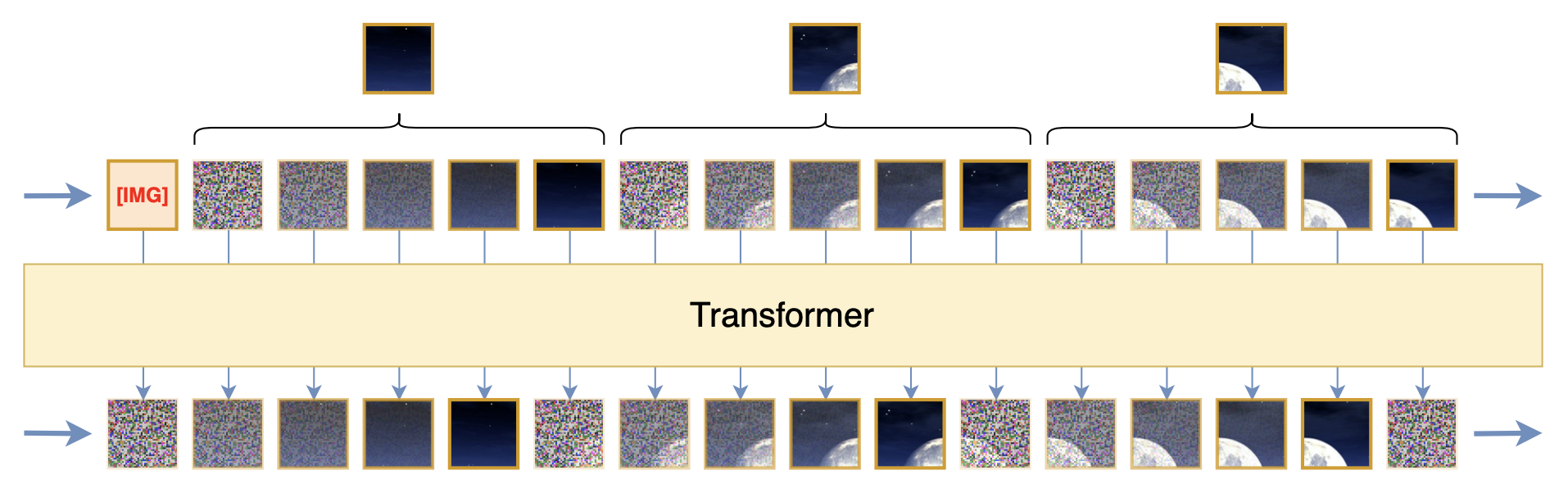Extending each patch by adding noise, making squared error a viable loss function

Readers familiar with diffusion models will quickly realize: constructing a gradually-changing sequence via noise addition, then training a recursive denoising model with squared error as the loss—isn't that just a diffusion model? Indeed—diffusion models' core idea is precisely "making squared error a valid loss function through progressive noise addition," and the scheme above borrows exactly this idea. Of course, the differences from a standard diffusion model are also obvious: e.g., a diffusion model adds noise to the whole image, whereas here we add noise to a patch; a diffusion model models $p(x_t|x_{t-1})$, whereas here we model $p(x_t|x_{< t})$, and so on. In its final form, what's proposed here is a scheme that combines diffusion modeling with autoregressive image learning.

The Efficiency Problem

Extending the sequence via noise addition so that plain squared error becomes usable, thereby making autoregressive image learning essentially consistent with our original plan (just with an added noise-injection step on the input)—this is undeniably a very satisfying result. However, things aren't quite so rosy: this scheme has at least two major issues, both of which can be summarized under a single word—efficiency.

First is the learning efficiency problem. We already discussed this in the very first post on diffusion models, Generative Diffusion Models Explained (Part 1): DDPM = Demolition + Construction]. The gist is that the training objective of predicting the noisy image at step $t$ from the noisy image at step $t-1$ requires double sampling over the noise, which leads to greater training variance, and thus requires more training steps to bring that variance down. After a series of variance-reduction tricks, we found that a more efficient approach is to directly predict the original image (or, equivalently, its difference from the original image):

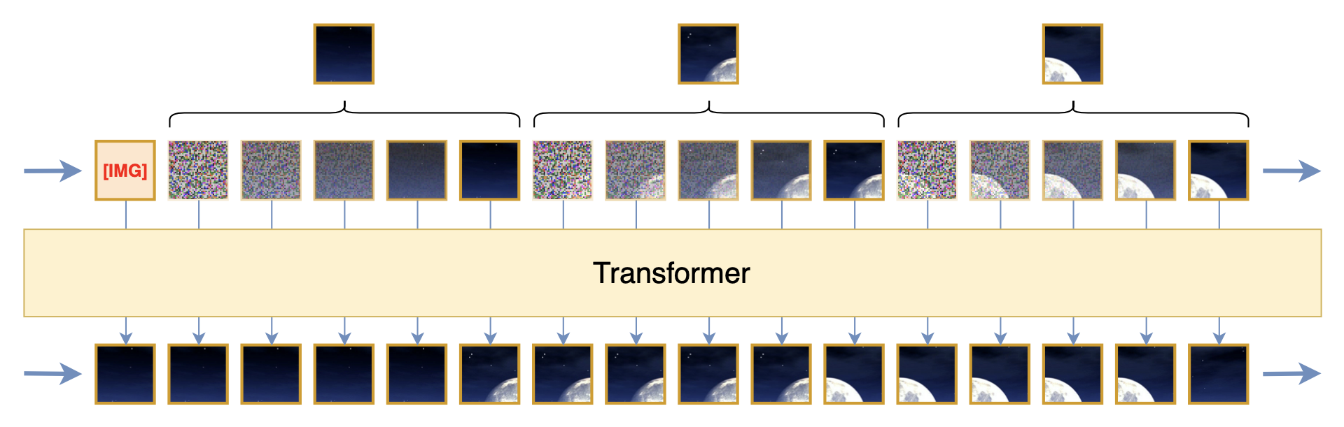Compared with predicting the next-step noisy image, directly predicting the original image is more efficient

Some readers might be confused: didn't we just say that the original, noise-free image doesn't follow a Gaussian distribution, so squared error shouldn't apply? This isn't so easy to explain intuitively—we can think of it as a fortunate coincidence of the Gaussian distribution, where squared error still turns out to be usable. For a more rigorous explanation, see Generative Diffusion Models Explained (Part 3): DDPM = Bayes + Denoising] and Generative Diffusion Models Explained (Part 4): DDIM = A High-Level View of DDPM].

Second is the computational efficiency problem. This one is easy to understand: if noise addition turns each patch into $T$ patches, the sequence length grows by a factor of $T$, which significantly increases both training and inference cost. Moreover, in theory, the noisy patches don't provide any real benefit to image understanding—keeping only the single clean, noise-free patch should in principle achieve the same effect. In other words, this scheme introduces a large amount of redundant input and computation as far as image understanding is concerned.

There are two possible approaches to solving this problem, which we'll go through one by one.

Separating Out Diffusion

If we insist on solving this within a single Transformer, we can consider adding a mask to attention, which breaks down into two parts. First, diffusion theory and practice tell us that predicting $x_t$ only requires $x_{t-1}$—we can ignore earlier inputs—meaning that different noisy versions of the same patch don't need to attend to each other. Second, to reduce redundancy, when predicting between different patches, or predicting subsequent text tokens, we only need to attend to the clean, noise-free patches. This yields an attention mask roughly like the following:

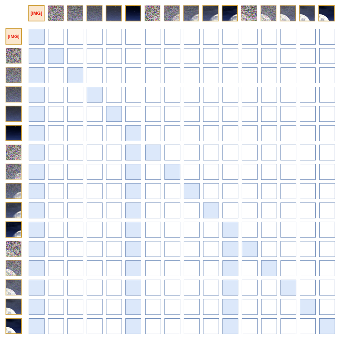An attention mask designed with the aim of simplifying the model and removing redundancy

Since this attention mask has a fixed sparse pattern, there's a lot of room for speeding it up. And since the noisy patches' attention computations are independent of each other, during training we don't need to compute all $T-1$ noisy patches at once—we can just sample a subset each time. Of course, this is still only a rough sketch; in practice there are details that need careful consideration, such as the fact that noisy patches have essentially no relation to one another, so their positional encoding needs to be designed separately, and so on—we won't go into that here.

If we allow two separate models to be chained together (while still training end-to-end), we can also split the diffusion model out entirely: the Transformer only handles the clean, noise-free patches, and the Transformer's output serves as the condition for the diffusion model, as shown below:

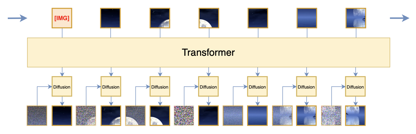Separating out the diffusion model, with the Transformer's output serving as the conditioning input for diffusion

This is roughly the scheme proposed in Kaiming's recent work Autoregressive Image Generation without Vector Quantization], though it was actually proposed earlier in Denoising Autoregressive Representation Learning]. Its benefit is that it keeps the Transformer part purer and more elegant, while also saving on computation, because: (1) the separated-out diffusion model can be made smaller; (2) for the diffusion model part, we can follow the usual training strategy of sampling just one noise step at a time. From the loss-function perspective, this amounts to using an extra diffusion model as the loss for predicting the next patch, thereby resolving the shortcomings of squared error.

Generation Direction

Earlier we mentioned that the two key issues in autoregressive learning for images are "patch splitting and ordering" and "the loss function." We just spent four sections barely getting the loss function issue somewhat straightened out, and even that could only be considered as having just touched the threshold. However, we are now going to find an even more pessimistic result — for the "patch splitting and ordering" problem, we can barely even touch the threshold.

From the perspective of the ultimate goal, "patch splitting and ordering" is meant to establish a generation sequence and direction for autoregressive learning; it consists of two steps, "splitting into patches" and "ordering." We also call "splitting into patches" Patchify. In the narrow sense, Patchify is simply a reshape-and-transpose operation on the pixel array: an array of shape $w\times h\times 3$ is first reshaped into $s\times (w/s) \times t\times (h/t)\times 3$, then transposed into $s\times t\times (w/s)\times (h/t)\times 3$, and finally reshaped into $s\times t\times (3wh/st)$. But in a broader sense, Patchify can refer to any scheme that turns an image array of shape $w\times h \times 3$ into an array of shape $s\times t\times d$ (where $s < w, t < h$), such as Stable Diffusion's Encoder encoding an image into a latent, or various VQ-Tokenizers turning an image into discrete IDs — these all count as Patchify in the broad sense.

"Ordering" is easier to understand. We know images have two directions (dimensions), "height" and "width," and the output features of most Patchify methods still retain this two-dimensional nature, whereas autoregressive generation is unidirectional, so a generation order needs to be specified. Common orderings include: 1) left-to-right then top-to-bottom, 2) spiraling from the center outward, 3) a "Z" pattern starting from the top-left corner, and so on. These ordering designs have a long history — they trace back to the first generation of image autoregressive models, i.e., autoregressive models operating directly on image pixels, such as the aforementioned PixelRNN/PixelCNN.

Naive Patchify and two different ordering schemes

Overall, "patch splitting and ordering" is the process of deconstructing an image into a one-dimensional sequence suitable for autoregressive learning — put more plainly, converting an image from a two-dimensional sequence into a one-dimensional one. So from the broadest possible perspective, the sequence of noisy images at different noise levels constructed by diffusion models, and the multi-scale sequence from Visual Autoregressive Modeling: Scalable Image Generation via Next-Scale Prediction, can both be classified under this umbrella. So, now that we've mentioned several different schemes for deconstructing images, a natural question arises: which scheme is better? What's the criterion for judging?

World Models

To answer this question, we first need to clarify what the fundamental difficulty of image generation — or rather, visual generation — actually is. In "Reinventing the Wheel" on Multimodality (I): Lossless Input, we briefly mentioned that the difficulty of image generation lies in the difficulty of continuous probability modeling. But actually, this is a very superficial judgment — if that were really all there was to it, the situation would be much more optimistic, since we've already developed quite a few continuous generative models such as diffusion models. In reality, the difficulty here runs far deeper than we might imagine...

What we call "images" can broadly be divided into two categories: pictures created by humans, and photographs taken by cameras. Since the proliferation of cameras and smartphones, images on the internet are in fact now dominated by photographs, so image generation is essentially equivalent to photograph generation. What is a photograph? It is a record of light — the projection of light from the three-dimensional world onto a two-dimensional plane. And what is light? Light is an electromagnetic wave, and electromagnetic waves are solutions to Maxwell's equations! From this line of thought we arrive at an undeniable fact: a real natural photograph is, in essence, a solution to Maxwell's equations. This means that perfect image generation is unavoidably bound up with the laws of physics — the very foundations of the world that so many theoretical physicists tirelessly pursue!

Coincidentally, ever since Sora appeared, we've often evaluated the quality of model-generated videos by asking "does it conform to the physical laws of the real world?" In fact, seemingly much simpler image generation can also be evaluated along this dimension of "conforming to physical laws" — for instance, the distribution of light and shadow in an image. It's just that with video, on top of optics (electromagnetism) there's now also dynamics added into the mix. If we keep brainstorming along this chain of thought, it becomes increasingly stunning, even unsettling, because it's equivalent to saying that a perfect visual generative model is, in effect, numerically simulating all sorts of physical laws — or, put more dramatically, it is actually simulating the evolution of the entire world, the entire universe. It is, in essence, a world model. This is no longer something that can be described as merely "hellishly difficult" — this is difficulty on the level of creating the universe.

Some readers might object: Maxwell's equations are hard, sure, but weren't they discovered by humans after all? We've also discovered even harder physical laws, such as quantum mechanics and general relativity, and we're continually getting closer to the ultimate theory (grand unification). So doesn't that mean the difficulty here isn't really so high? No — don't get confused here. Even if we truly could discover the completely correct laws of physics, that is an entirely different matter from having the ability to "numerically simulate using these laws." For instance, we might be able to write down an equation by hand, but that doesn't mean we can solve it by hand. So the fact that we can discover physical laws doesn't mean we're capable of using those laws to derive or simulate the real world. To put it more concretely: right now we can sit here and say that a photograph is, in essence, a solution to Maxwell's equations, but no one is able to hand-draw a photograph.

(Note: This chain of thinking originated from the idea that "an image is essentially a solution to Maxwell's equations," which my team lead Zhou Xinyu shared with me during a technical discussion. The first time I heard this seemingly absurd but ultimately unavoidable viewpoint, I was stunned and shaken — I suddenly felt as though I had grasped the essential difficulty of multimodal models.)

Human Values

Overall, what this brainstorm is trying to express is that a truly perfect visual generative model would be, in the fullest sense, a world model, and its difficulty is on the order of creating the universe. So do we want to create the universe? Are we capable of creating the universe? I believe that, within any imaginable timeframe, the answer to both is no — after all, that would essentially mean pitting human effort against the entire universe. So the key here is to abandon the notion of "perfection." Just as a human cannot hand-draw a photograph, this doesn't stop humans from painting, nor does it stop humans from conveying information through drawing. Likewise, when we judge whether a model-generated video conforms to the laws of physics, we're not actually measuring the trajectories in the video and plugging them into physical formulas — we're simply relying on visual inspection combined with our intuitive sense of physical laws.

To put it bluntly: it's fine to be lossy, as long as it's lossless with respect to human values. So what does this have to do with the "patch splitting and ordering" issue discussed earlier? As we said at the very beginning, autoregressive learning doesn't just endow the model with generative ability — it also serves as an unsupervised learning pathway to improve the model's comprehension ability (if you can't generate, you don't understand). If we had a model with truly unlimited fitting power (world-creating power), then all "patch splitting and ordering" schemes would be equivalent, because the exact joint distribution doesn't depend on how the random variables are factorized. Unfortunately, we don't have such a model, so we have no choice but to make trade-offs.

Note that we want to use learning-to-generate to promote understanding, and here "understanding" must necessarily be aligned with human visual understanding — that is the very purpose of training AI. However, none of the "patch splitting and ordering" schemes listed earlier match the way humans actually understand images visually. To put it more directly: human understanding of an image is not left-to-right or top-to-bottom, nor is it center-to-periphery or a "Z" pattern; in fact, human understanding of images isn't even organized in units of patches, and it certainly isn't the gradual-noising process used by diffusion. If we use any of the existing "patch splitting and ordering" schemes for autoregressive learning, we may indeed have a chance at endowing the model with some degree of visual generation ability, but since these image deconstruction methods fundamentally don't match how humans understand images visually, it's hard to believe that this kind of autoregressive learning can actually promote the model's visual understanding ability — or, more precisely, it's hard for it to promote the model's ability to mimic human visual understanding.

The main reason for this difficulty is that an image is a "result," not a "process." Take human-created images, for example — whether hand-drawn or edited in Photoshop, the process happens step by step, but what's ultimately presented is an image that conceals its own creative process. This is different from text: although we don't know exactly how a writer conceived of a given passage, we do know that most people write from left to right, so the text itself already encodes its creation (writing) process. But what about a painting? Looking at a painting, can we tell which area or which brushstroke the painter did first? Clearly not — and that's exactly why most people can write but cannot replicate a painting by copying it. Thinking about it even more deeply, this could be understood as humans being generally better at imitating along the temporal dimension than along the spatial dimension, because there's only one temporal dimension while there are three spatial dimensions — the latter simply has too much freedom.

For now, it seems there's only one rather "compromised" way to address this problem: use as much image-text data as possible that aligns with human values (and of course, other valuable supervisory signals for images could work too) to supervisedly train a "patch splitting and ordering" model. Note that unlike a typical Vision Encoder, this model needs to directly output a one-dimensional sequence rather than preserving the two-dimensional nature of the image, which eliminates the need for a subsequent ordering step. For the model design, we can refer to TiTok (this is the third time we've mentioned TiTok), which essentially uses cross attention to convert a two-dimensional sequence into a one-dimensional one; besides that, Q-Former can achieve a similar effect. In short, there won't be too much difficulty on the model design side — the core work shifts to the data engineering of image-text pairs.

But given this, how far the model can go becomes uncertain, because we originally hoped to use autoregressive learning to promote the model's understanding ability, yet now autoregressive learning depends on an Encoder trained via a comprehension task. In the ideal case, these two models would mutually reinforce and co-evolve; but in the non-ideal case, the model's capability would be bottlenecked by the quantity and quality of the supervised data used to train the Encoder, and we would fail to achieve true unsupervised learning after all.

Summary

This article continues "reinventing the wheel" with some thoughts on multimodal learning, mainly revolving around autoregressive learning for vision. The general content is:

1. Autoregressive learning both endows the model with generative ability and serves as an unsupervised learning pathway that promotes comprehension ability through generation;
2. For images, the question is not whether to do autoregression, but how to do autoregression more effectively;
3. When feeding images in as continuous features, autoregressive learning faces two major difficulties: patch splitting and ordering, and the loss function;
4. The loss function shouldn't simply be squared error — instead, one could consider appending a small diffusion model to predict the next patch;
5. "Patch splitting and ordering" is the fundamental difficulty of image autoregressive learning, and the choice made here determines whether autoregressive learning can truly promote understanding;
6. Perfect image/visual generation inevitably has to connect with physical laws, thereby constituting a "world model";
7. But a world model is hard to achieve, so choosing a "patch splitting and ordering" scheme that aligns with human values becomes especially important;
8. In the end, it seems we can only "compromise" by using supervised learning to obtain a "patch splitting and ordering" model aligned with human values.

There may be quite a few "wild claims" and "fallacies" in here — please judge for yourselves and forgive me where needed. The main purpose of writing these thoughts down is so that, someday in the future, I can look back and see how feasible — or how laughable — my original ideas turned out to be.