Generative Diffusion Models Explained (II): DDPM = Autoregressive VAE
In the article Generative Diffusion Models Explained (I): DDPM = Demolition + Construction, we built a colorful analogy of "demolition and construction" for the generative diffusion model DDPM, and used this analogy to give a complete derivation of its theoretical form. In that article, we also pointed out that DDPM is, in essence, no longer a traditional diffusion model — it is really more of a variational autoencoder (VAE). Indeed, the original DDPM paper itself derives the model along VAE lines.
So in this post, let's re-introduce DDPM from the VAE point of view, and along the way share my own Keras implementation and some practical experience.
Breaking Through with Multiple Steps
In a traditional VAE, both the encoding process and the generation process are done in a single step:
\begin{equation}\text{encoding:}\,\,x\to z\,,\quad \text{generate:}\,\,z\to x\end{equation}more
This setup involves only three distributions: the encoding distribution $p(z|x)$, the generative distribution $q(x|z)$, and the prior distribution $q(z)$. Its advantage is a simple form, and the mapping between $x$ and $z$ is fairly deterministic, so we can obtain both an encoder and a generator at once, enabling things like latent-variable editing. But its drawback is also obvious: because our ability to model probability distributions is limited, all three of these distributions can only be modeled as Gaussians, which caps the model's expressive power and typically leads to blurry generation results.
To break through this limitation, DDPM decomposes the encoding and generation processes into $T$ steps:
\begin{equation}\begin{aligned}&\text{encoding:}\,\,\boldsymbol{x} = \boldsymbol{x}_0 \to \boldsymbol{x}_1 \to \boldsymbol{x}_2 \to \cdots \to \boldsymbol{x}_{T-1} \to \boldsymbol{x}_T = \boldsymbol{z} \\ &\text{generate:}\,\,\boldsymbol{z} = \boldsymbol{x}_T \to \boldsymbol{x}_{T-1} \to \boldsymbol{x}_{T-2} \to \cdots \to \boldsymbol{x}_1 \to \boldsymbol{x}_0 = \boldsymbol{x} \end{aligned}\label{eq:factor}\end{equation}
In this way, each $p(\boldsymbol{x}_t|\boldsymbol{x}_{t-1})$ and $q(\boldsymbol{x}_{t-1}|\boldsymbol{x}_t)$ is only responsible for modeling a tiny change, and they are still modeled as Gaussians. At this point you might ask: if they're still Gaussians, why would splitting into multiple steps be any better than a single step? The reason is that for a small enough change, a Gaussian can approximate it arbitrarily well — much like a curve can be approximated by a straight line over a small enough range. Decomposing into many steps is a bit like fitting a complicated curve with a piecewise-linear function, so in principle it can surpass the fitting capacity limits of a traditional single-step VAE.
Joint Divergence
So the plan now is to strengthen the traditional VAE by recursively decomposing $\eqref{eq:factor}$: each encoding step is modeled as $p(\boldsymbol{x}_t|\boldsymbol{x}_{t-1})$, and each generation step is modeled as $q(\boldsymbol{x}_{t-1}|\boldsymbol{x}_t)$. The corresponding joint distributions are:
\begin{equation}\begin{aligned}&p(\boldsymbol{x}_0, \boldsymbol{x}_1, \boldsymbol{x}_2, \cdots, \boldsymbol{x}_T) = p(\boldsymbol{x}_T|\boldsymbol{x}_{T-1})\cdots p(\boldsymbol{x}_2|\boldsymbol{x}_1) p(\boldsymbol{x}_1|\boldsymbol{x}_0) \tilde{p}(\boldsymbol{x}_0) \\ &q(\boldsymbol{x}_0, \boldsymbol{x}_1, \boldsymbol{x}_2, \cdots, \boldsymbol{x}_T) = q(\boldsymbol{x}_0|\boldsymbol{x}_1)\cdots q(\boldsymbol{x}_{T-2}|\boldsymbol{x}_{T-1}) q(\boldsymbol{x}_{T-1}|\boldsymbol{x}_T) q(\boldsymbol{x}_T) \end{aligned}\end{equation}
Don't forget that $\boldsymbol{x}_0$ represents the real sample, so $\tilde{p}(\boldsymbol{x}_0)$ is the data distribution; and $\boldsymbol{x}_T$ represents the final encoding, so $q(\boldsymbol{x}_T)$ is the prior distribution. The remaining $p(\boldsymbol{x}_t|\boldsymbol{x}_{t-1})$ and $q(\boldsymbol{x}_{t-1}|\boldsymbol{x}_t)$ represent a small step of encoding and generation respectively. (Note: After some deliberation, I've decided to stick with the notation convention this site has always used for VAEs, namely "the encoding distribution is written $p$, the generative distribution is written $q$." So here, $p$ and $q$ have exactly the opposite meaning to the ones in the DDPM paper — readers should keep this in mind.)
In Variational Autoencoders (II): From a Bayesian Perspective, I argued that the cleanest theoretical way to understand a VAE is as minimizing the KL divergence between two joint distributions. The same holds for DDPM: having written out the two joint distributions above, the goal of DDPM is to minimize
\begin{equation}KL(p\Vert q) = \int p(\boldsymbol{x}_T|\boldsymbol{x}_{T-1})\cdots p(\boldsymbol{x}_1|\boldsymbol{x}_0) \tilde{p}(\boldsymbol{x}_0) \log \frac{p(\boldsymbol{x}_T|\boldsymbol{x}_{T-1})\cdots p(\boldsymbol{x}_1|\boldsymbol{x}_0) \tilde{p}(\boldsymbol{x}_0)}{q(\boldsymbol{x}_0|\boldsymbol{x}_1)\cdots q(\boldsymbol{x}_{T-1}|\boldsymbol{x}_T) q(\boldsymbol{x}_T)} d\boldsymbol{x}_0 d\boldsymbol{x}_1\cdots d\boldsymbol{x}_T\label{eq:kl}\end{equation}
This is DDPM's optimization objective. Everything up to this point matches the results of the original DDPM paper (just with slightly different notation), and is also consistent with the earlier paper Deep Unsupervised Learning using Nonequilibrium Thermodynamics. Next, we need to pin down concrete forms for $p(\boldsymbol{x}_t|\boldsymbol{x}_{t-1})$ and $q(\boldsymbol{x}_{t-1}|\boldsymbol{x}_t)$, and then simplify DDPM's optimization objective $\eqref{eq:kl}$.
Divide and Conquer
First, we should note that DDPM only aims to be a generative model, so it models each encoding step as an extremely simple Gaussian: $p(\boldsymbol{x}_t|\boldsymbol{x}_{t-1})=\mathcal{N}(\boldsymbol{x}_t;\alpha_t \boldsymbol{x}_{t-1}, \beta_t^2 \boldsymbol{I})$, whose distinguishing feature is that the mean vector is simply the input $\boldsymbol{x}_{t-1}$ scaled by a scalar $\alpha_t$. By contrast, in a traditional VAE both the mean and variance are learned by a neural network. So DDPM gives up the model's encoding capability, ending up as a purely generative model. As for $q(\boldsymbol{x}_{t-1}|\boldsymbol{x}_t)$, it is modeled as a Gaussian $\mathcal{N}(\boldsymbol{x}_{t-1};\boldsymbol{\mu}(\boldsymbol{x}_t), \sigma_t^2 \boldsymbol{I})$ with a learnable mean vector. Here $\alpha_t,\beta_t,\sigma_t$ are not trainable parameters but preset values (we'll discuss how to set them later), so the only trainable parameters in the whole model are $\boldsymbol{\mu}(\boldsymbol{x}_t)$. (Note: the definition of $\alpha_t,\beta_t$ in this article differs from the original paper.)
Since the distribution $p$ currently contains no trainable parameters, integrating over $p$ in the objective $\eqref{eq:kl}$ only contributes a negligible constant. So the objective $\eqref{eq:kl}$ is equivalent to
\begin{equation}\begin{aligned}&\,-\int p(\boldsymbol{x}_T|\boldsymbol{x}_{T-1})\cdots p(\boldsymbol{x}_1|\boldsymbol{x}_0) \tilde{p}(\boldsymbol{x}_0) \log q(\boldsymbol{x}_0|\boldsymbol{x}_1)\cdots q(\boldsymbol{x}_{T-1}|\boldsymbol{x}_T) q(\boldsymbol{x}_T) d\boldsymbol{x}_0 d\boldsymbol{x}_1\cdots d\boldsymbol{x}_T \\ =&\,-\int p(\boldsymbol{x}_T|\boldsymbol{x}_{T-1})\cdots p(\boldsymbol{x}_1|\boldsymbol{x}_0) \tilde{p}(\boldsymbol{x}_0) \left[\log q(\boldsymbol{x}_T) + \sum_{t=1}^T\log q(\boldsymbol{x}_{t-1}|\boldsymbol{x}_t)\right] d\boldsymbol{x}_0 d\boldsymbol{x}_1\cdots d\boldsymbol{x}_T \end{aligned}\end{equation}
Since the prior distribution $q(\boldsymbol{x}_T)$ is generally taken to be a standard normal distribution, which also has no parameters, this term likewise contributes only a constant. So what we actually need to compute is each term
\begin{equation}\begin{aligned}&\,-\int p(\boldsymbol{x}_T|\boldsymbol{x}_{T-1})\cdots p(\boldsymbol{x}_1|\boldsymbol{x}_0) \tilde{p}(\boldsymbol{x}_0) \log q(\boldsymbol{x}_{t-1}|\boldsymbol{x}_t) d\boldsymbol{x}_0 d\boldsymbol{x}_1\cdots d\boldsymbol{x}_T\\ =&\,-\int p(\boldsymbol{x}_t|\boldsymbol{x}_{t-1})\cdots p(\boldsymbol{x}_1|\boldsymbol{x}_0) \tilde{p}(\boldsymbol{x}_0) \log q(\boldsymbol{x}_{t-1}|\boldsymbol{x}_t) d\boldsymbol{x}_0 d\boldsymbol{x}_1\cdots d\boldsymbol{x}_t\\ =&\,-\int p(\boldsymbol{x}_t|\boldsymbol{x}_{t-1})p(\boldsymbol{x}_{t-1}|\boldsymbol{x}_0) \tilde{p}(\boldsymbol{x}_0) \log q(\boldsymbol{x}_{t-1}|\boldsymbol{x}_t) d\boldsymbol{x}_0 d\boldsymbol{x}_{t-1}d\boldsymbol{x}_t \end{aligned}\end{equation}
Here, the first equality holds because $q(\boldsymbol{x}_{t-1}|\boldsymbol{x}_t)$ depends at most on $\boldsymbol{x}_t$, so integrating over the distribution from $t+1$ to $T$ just gives 1; the second equality holds because $q(\boldsymbol{x}_{t-1}|\boldsymbol{x}_t)$ also doesn't depend on $\boldsymbol{x}_1,\cdots,\boldsymbol{x}_{t-2}$, so we can pre-compute the integral over them, giving the result $p(\boldsymbol{x}_{t-1}|\boldsymbol{x}_0)=\mathcal{N}(\boldsymbol{x}_{t-1};\bar{\alpha}_{t-1} \boldsymbol{x}_0, \bar{\beta}_{t-1}^2 \boldsymbol{I})$ — see equation $\eqref{eq:x0-xt}$ in the next section for reference.
Déjà Vu
The rest of the derivation is basically identical to the "How Do We Build It, Then?" section of the previous article:
1. Discarding constants irrelevant to optimization, the term $-\log q(\boldsymbol{x}_{t-1}|\boldsymbol{x}_t)$ contributes $\frac{1}{2\sigma_t^2}\left\Vert\boldsymbol{x}_{t-1} - \boldsymbol{\mu}(\boldsymbol{x}_t)\right\Vert^2$;
2. $p(\boldsymbol{x}_{t-1}|\boldsymbol{x}_0)$ implies $\boldsymbol{x}_{t-1} = \bar{\alpha}_{t-1}\boldsymbol{x}_0 + \bar{\beta}_{t-1}\bar{\boldsymbol{\varepsilon}}_{t-1}$, and $p(\boldsymbol{x}_t|\boldsymbol{x}_{t-1})$ in turn implies $\boldsymbol{x}_t = \alpha_t \boldsymbol{x}_{t-1} + \beta_t \boldsymbol{\varepsilon}_t$, where $\bar{\boldsymbol{\varepsilon}}_{t-1},\boldsymbol{\varepsilon}_t\sim \mathcal{N}(\boldsymbol{0},\boldsymbol{I})$;
3. $\boldsymbol{x}_{t-1} = \frac{1}{\alpha_t}\left(\boldsymbol{x}_t - \beta_t \boldsymbol{\varepsilon}_t\right)$ then motivates us to parameterize $\boldsymbol{\mu}(\boldsymbol{x}_t)$ as $\boldsymbol{\mu}(\boldsymbol{x}_t) = \frac{1}{\alpha_t}\left(\boldsymbol{x}_t - \beta_t \boldsymbol{\epsilon}_{\boldsymbol{\theta}}(\boldsymbol{x}_t, t)\right)$.
After this series of transformations, the optimization objective becomes equivalent to
\begin{equation}\frac{\beta_t^2}{\alpha_t^2\sigma_t^2}\mathbb{E}_{\bar{\boldsymbol{\varepsilon}}_{t-1},\boldsymbol{\varepsilon}_t\sim \mathcal{N}(\boldsymbol{0},\boldsymbol{I}),\boldsymbol{x}_0\sim \tilde{p}(\boldsymbol{x}_0)}\left[\left\Vert \boldsymbol{\varepsilon}_t - \boldsymbol{\epsilon}_{\boldsymbol{\theta}}(\bar{\alpha}_t\boldsymbol{x}_0 + \alpha_t\bar{\beta}_{t-1}\bar{\boldsymbol{\varepsilon}}_{t-1} + \beta_t \boldsymbol{\varepsilon}_t, t)\right\Vert^2\right]\end{equation}
Then, following the change of variables in the "Reducing Variance" section, we get
\begin{equation}\frac{\beta_t^4}{\bar{\beta}_t^2\alpha_t^2\sigma_t^2}\mathbb{E}_{\boldsymbol{\varepsilon}\sim \mathcal{N}(\boldsymbol{0},\boldsymbol{I}),\boldsymbol{x}_0\sim \tilde{p}(\boldsymbol{x}_0)}\left[\left\Vert\boldsymbol{\varepsilon} - \frac{\bar{\beta}_t}{\beta_t}\boldsymbol{\epsilon}_{\boldsymbol{\theta}}(\bar{\alpha}_t\boldsymbol{x}_0 + \bar{\beta}_t\boldsymbol{\varepsilon}, t)\right\Vert^2\right]\label{eq:loss}\end{equation}
This is exactly DDPM's training objective (the original paper found experimentally that dropping the coefficient in front of the expression above works even better in practice). We arrived at it starting from the VAE optimization objective and progressively simplifying the resulting integrals. It's a bit long, but every step follows a clear logic — computationally involved, but not conceptually mysterious.
By contrast, the original DDPM paper rather abruptly introduces a quantity $q(\boldsymbol{x}_{t-1}|\boldsymbol{x}_t,\boldsymbol{x}_0)$ (the paper's own notation) to perform a telescoping cancellation, and then converts the result into the KL-divergence form of two Gaussians. This step is, in my opinion, far too much of a trick, feeling rather "out of nowhere" — something I personally find quite hard to accept.
Setting the Hyperparameters
In this section, let's discuss how to choose $\alpha_t,\beta_t,\sigma_t$.
For $p(\boldsymbol{x}_t|\boldsymbol{x}_{t-1})$, it's conventional to set $\alpha_t^2 + \beta_t^2=1$, which cuts the number of parameters in half and helps simplify the form. We already derived this in the previous article: because of the additivity of Gaussians, under this constraint we have
\begin{equation}p(\boldsymbol{x}_t|\boldsymbol{x}_0) = \int p(\boldsymbol{x}_t|\boldsymbol{x}_{t-1})\cdots p(\boldsymbol{x}_1|\boldsymbol{x}_0) d\boldsymbol{x}_1\cdots d\boldsymbol{x}_{t-1} = \mathcal{N}(\boldsymbol{x}_t;\bar{\alpha}_t \boldsymbol{x}_0, \bar{\beta}_t^2 \boldsymbol{I})\label{eq:x0-xt}\end{equation}
where $\bar{\alpha}_t = \alpha_1\cdots\alpha_t$ and $\bar{\beta}_t = \sqrt{1-\bar{\alpha}_t^2}$, so that $p(\boldsymbol{x}_t|\boldsymbol{x}_0)$ takes on a fairly compact form. You might wonder how one would think of the constraint $\alpha_t^2 + \beta_t^2=1$ in the first place. We know $\mathcal{N}(\boldsymbol{x}_t;\alpha_t \boldsymbol{x}_{t-1}, \beta_t^2 \boldsymbol{I})$ implies $\boldsymbol{x}_t = \alpha_t \boldsymbol{x}_{t-1} + \beta_t \boldsymbol{\varepsilon}_t,\boldsymbol{\varepsilon}_t\sim \mathcal{N}(\boldsymbol{0},\boldsymbol{I})$; if $\boldsymbol{x}_{t-1}$ is also $\sim \mathcal{N}(\boldsymbol{0},\boldsymbol{I})$, then we would want $\boldsymbol{x}_t$ to also be $\sim \mathcal{N}(\boldsymbol{0},\boldsymbol{I})$, and that's exactly what pins down $\alpha_t^2+\beta_t^2=1$.
As mentioned earlier, $q(\boldsymbol{x}_T)$ is generally taken to be the standard normal distribution $\mathcal{N}(\boldsymbol{x}_T;\boldsymbol{0}, \boldsymbol{I})$. Since our learning goal is to minimize the KL divergence between the two joint distributions, i.e., we want $p=q$, their marginal distributions should naturally be equal too, so we also want
\begin{equation}q(\boldsymbol{x}_T) = \int p(\boldsymbol{x}_T|\boldsymbol{x}_{T-1})\cdots p(\boldsymbol{x}_1|\boldsymbol{x}_0) \tilde{p}(\boldsymbol{x}_0) d\boldsymbol{x}_0 d\boldsymbol{x}_1\cdots d\boldsymbol{x}_{T-1} = \int p(\boldsymbol{x}_T|\boldsymbol{x}_0) \tilde{p}(\boldsymbol{x}_0) d\boldsymbol{x}_0 \end{equation}
Since the data distribution $\tilde{p}(\boldsymbol{x}_0)$ is arbitrary, for this equation to hold identically we must have $p(\boldsymbol{x}_T|\boldsymbol{x}_0)=q(\boldsymbol{x}_T)$ degenerate into a standard normal distribution independent of $\boldsymbol{x}_0$. This means we need to design $\alpha_t$ appropriately so that $\bar{\alpha}_T\approx 0$ holds. This again tells us that DDPM has no encoding capability: the final $p(\boldsymbol{x}_T|\boldsymbol{x}_0)$ can be said to be independent of the input $\boldsymbol{x}_0$. In terms of the "demolition-construction" analogy from the previous article: the original building has been completely demolished into raw materials, and if we rebuild using this pile of materials, we could construct a building of any shape — not necessarily the shape it had before demolition. DDPM chooses $\alpha_t = \sqrt{1 - \frac{0.02t}{T}}$; we already analyzed the properties of this choice in the "Setting the Hyperparameters" section of the previous article.
As for $\sigma_t$, in theory different data distributions $\tilde{p}(\boldsymbol{x}_0)$ correspond to different optimal choices of $\sigma_t$. But since we don't want to make $\sigma_t$ a trainable parameter, we instead choose some special cases of $\tilde{p}(\boldsymbol{x}_0)$ to derive the corresponding optimal $\sigma_t$, and assume that the $\sigma_t$ derived from these special cases generalizes to arbitrary data distributions. We can consider two simple examples:
1. Suppose the training set consists of a single sample $\boldsymbol{x}_*$, i.e., $\tilde{p}(\boldsymbol{x}_0)$ is a Dirac distribution $\delta(\boldsymbol{x}_0 - \boldsymbol{x}_*)$; one can then derive the optimal $\sigma_t = \frac{\bar{\beta}_{t-1}}{\bar{\beta}_t}\beta_t$;
2. Suppose the data distribution $\tilde{p}(\boldsymbol{x}_0)$ follows a standard normal distribution; one can then derive the optimal $\sigma_t = \beta_t$.
Experimental results show that these two choices perform similarly, so either one can be used for sampling. The derivations for both results are somewhat lengthy, so we'll leave that discussion for another time.
Reference Implementation
A model this exciting deserves a Keras implementation! Here's my reference implementation:
GitHub: https://github.com/bojone/Keras-DDPM
Note that my implementation doesn't strictly follow the original open-source DDPM code; instead, I simplified the U-Net architecture based on my own design (for example, replacing feature concatenation with addition, removing attention, etc.) to get quick results. In testing, on a single 3090 with 24GB of GPU memory, training a 128×128 CelebA HQ face dataset with blocks=1,batch_size=64 started showing promising results within half a day. Here's the sampling result after 3 days of training:
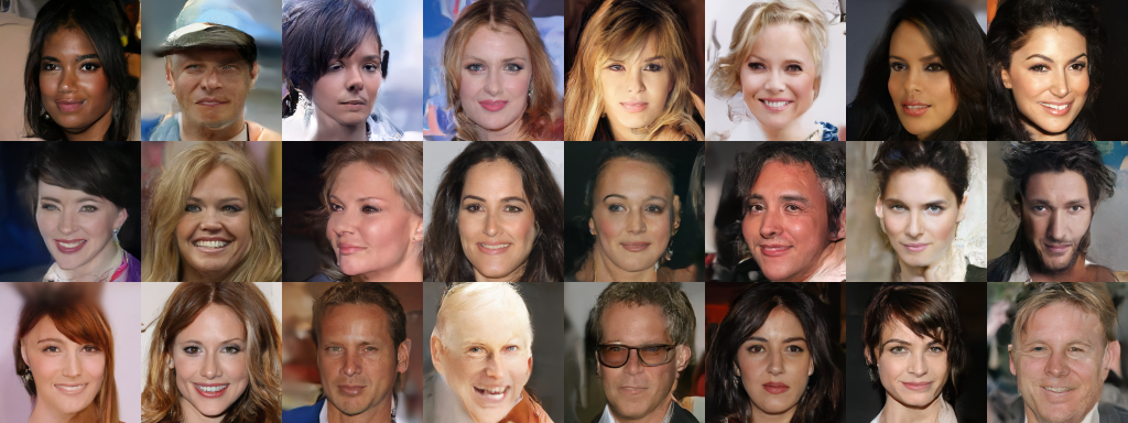 Demonstration of my trained DDPM's sampling results
During debugging, I accumulated the following practical experience:
1. The loss function must not be MSE, but rather squared Euclidean distance. The difference between the two is that MSE divides the squared Euclidean distance by the $\text{width}\times\text{high}\times\text{num channels}$ of the image, which makes the loss value too small — the gradients of some parameters may be rounded to zero, causing the training process to converge at first and then diverge. This phenomenon also frequently shows up in low-precision training; see Using Mixed Precision and XLA to Speed Up Training in bert4keras for reference.
2. For normalization, you can use Instance Norm, Layer Norm, Group Norm, etc., but avoid Batch Norm, since Batch Norm has a train/inference inconsistency problem that can cause training to look great while inference performs poorly.
3. There's no need to copy the network architecture from the original paper verbatim — that paper was written to chase state-of-the-art results, so its architecture is inevitably large and slow. Just design an autoencoder along U-Net lines, and you can basically get decent results, since this is essentially a pure regression problem, which is quite easy to train.
4. Regarding how to feed in the parameter $t$, the original paper used sinusoidal positional encoding. I found that simply switching to a trainable embedding gives about the same results.
5. Following my usual habits from pretraining language models, I used the LAMB optimizer, which makes it easier to tune the learning rate — basically, a learning rate of $10^{-3}$ works for training the model regardless of initialization scheme.
Overall Assessment
Combining Generative Diffusion Models Explained (I): DDPM = Demolition + Construction with this article, readers should now have formed their own view of DDPM, and can basically see its strengths, its weaknesses, and where the natural directions for improvement lie.
DDPM's strengths are obvious: it's easy to train, and the generated images are sharp. "Easy to train" here is relative to GANs — a GAN involves a $\min\text{-}\max$ process, with a lot of uncertainty during training and a tendency to collapse, whereas DDPM is purely a regression loss that just needs to be minimized directly, so training is very stable. At the same time, thanks to the "demolition-construction" analogy, we can see that DDPM is no less intuitive to understand than GANs.
That said, DDPM's drawbacks are equally obvious. The most prominent one is that sampling is very slow, requiring $T$ model evaluations (the original paper needed $T=1000$ to complete sampling) — that's roughly $T$ times slower than a GAN's one-shot sampling, and a lot of follow-up work has tried to improve on this. Second, in a GAN, the mapping from random noise to a generated sample is a deterministic transformation, so the random noise is a disentangled latent variable of the generated result — we can interpolate in this space, or edit it to achieve controllable generation. But in DDPM, the generation process is entirely stochastic, with no deterministic relationship between the two, so this kind of editable generation doesn't exist. The original DDPM paper does demonstrate an interpolation-based generation, but that's just interpolating between the original images, then using noise to blur the image so the model can "imagine" a new image — this kind of interpolation can hardly achieve semantically meaningful blending.
Beyond addressing the drawbacks above, there are other directions DDPM could be extended in. For instance, all the DDPM demonstrations so far are unconditional generation — it's natural to think of a conditional version of DDPM, just as VAE has C-VAE and GAN has C-GAN. This is in fact already a mainstream application of diffusion models today: for example, Google's Imagen uses diffusion models for both text-to-image generation and super-resolution, both of which are essentially conditional diffusion models. Another direction: current DDPM is designed for continuous variables, but conceptually the idea should also apply to discrete data — so how should we design a DDPM for discrete data?
Related Work
When it comes to work related to DDPM, most people think of traditional diffusion models, energy-based models, or denoising autoencoders. But what I want to bring up here is something else — something this blog covered before, and which one could even argue DDPM is a special case of: The Powerful NVAE: Never Again Say VAE-Generated Images Are Blurry.
From the VAE perspective, traditional VAEs tend to generate blurry images, while DDPM is (as far as I'm aware) only the second VAE capable of generating sharp images — the first being NVAE. Looking back at NVAE's formulation, we find it has a great deal in common with DDPM: NVAE also introduces a large number of latent variables $z=\{z_1,z_2,\dots,z_L\}$, which likewise form a recursive relationship, so NVAE's sampling process is quite similar to DDPM's.
In terms of theoretical form, DDPM can be seen as an extremely simplified NVAE: the recursive relationship among the latent variables is modeled purely as a Markov-chain of conditional Gaussians, rather than the non-Markovian structure of NVAE, and the generative model is just the same model applied repeatedly, rather than NVAE's approach of using one giant model that simultaneously leverages $z=\{z_1,z_2,\dots,z_L\}$. That said, when NVAE makes use of its many $z=\{z_1,z_2,\dots,z_L\}$, it also introduces a parameter-sharing mechanism, which achieves a similar effect to applying the same model repeatedly, albeit by a different route.
Summary
This article derived DDPM from the perspective of the variational autoencoder. From this viewpoint, DDPM is a simplified autoregressive VAE, quite similar to the earlier NVAE. Along the way, I also shared my own DDPM implementation and practical experience, and gave a fairly comprehensive assessment of DDPM.
Translated automatically with claude-sonnet-5; all equations are reproduced verbatim from the source. Copyright remains with the original author.