Random Talk on Generative Diffusion Models (Part 4): DDIM = DDPM from a Higher Vantage Point

生成扩散模型漫谈（四）：DDIM = 高观点DDPM 苏剑林 · 2022-07-27 · Machine Learning differential equation generative model DDPM diffusion

Many readers have probably heard of, or even read, Felix Klein's Elementary Mathematics from an Advanced Standpoint. As the name suggests, this is a body of work that, once one has learned deeper and more complete mathematics, revisits the elementary mathematics learned earlier from a higher vantage point, so as to arrive at a more comprehensive understanding — and sometimes even to gain new insight by reviewing the old. There are quite a few similar books, such as Revisiting Calculus and Visual Complex Analysis.

前言

回到扩散模型，目前我们已经通过三篇文章从不同视角去解读了DDPM，那么它是否也存在一个更高的理解视角，让我们能从中得到新的收获呢？当然有，《Denoising Diffusion Implicit Models》介绍的DDIM模型就是经典的案例，本文一起来欣赏它。

Analysis of the Approach

In Generative Diffusion Models Rambling (III): DDPM = Bayes + Denoising, we mentioned that the derivation introduced there is closely related to DDIM. Specifically, that derivation can be roughly summarized as follows:

\begin{equation}p(\boldsymbol{x}_t|\boldsymbol{x}_{t-1})\xrightarrow{\text{derivation}}p(\boldsymbol{x}_t|\boldsymbol{x}_0)\xrightarrow{\text{derivation}}p(\boldsymbol{x}_{t-1}|\boldsymbol{x}_t, \boldsymbol{x}_0)\xrightarrow{\text{approx}}p(\boldsymbol{x}_{t-1}|\boldsymbol{x}_t)\end{equation}more

The process unfolds step by step. However, we find that the final result has two notable features:

1. The loss function depends only on $p(\boldsymbol{x}_t|\boldsymbol{x}_0)$;
2. The sampling process depends only on $p(\boldsymbol{x}_{t-1}|\boldsymbol{x}_t)$.

That is to say, although the whole process was derived step by step starting from $p(\boldsymbol{x}_t|\boldsymbol{x}_{t-1})$, from the end result it looks like $p(\boldsymbol{x}_t|\boldsymbol{x}_{t-1})$ never actually mattered at all. So let's boldly indulge in a bit of "wishful thinking":

High-level perspective 1: Since the result doesn't depend on $p(\boldsymbol{x}_t|\boldsymbol{x}_{t-1})$, can we simply "kick away the ladder" and remove $p(\boldsymbol{x}_t|\boldsymbol{x}_{t-1})$ from the entire derivation process?

DDIM is exactly the product of this "wild imagination"!

Undetermined Coefficients

Some readers might think, based on Bayes' theorem used in the previous article,

\begin{equation}p(\boldsymbol{x}_{t-1}|\boldsymbol{x}_t, \boldsymbol{x}_0) = \frac{p(\boldsymbol{x}_t|\boldsymbol{x}_{t-1})p(\boldsymbol{x}_{t-1}|\boldsymbol{x}_0)}{p(\boldsymbol{x}_t|\boldsymbol{x}_0)}\end{equation}

How can we get $p(\boldsymbol{x}_{t-1}|\boldsymbol{x}_t, \boldsymbol{x}_0)$ without a given $p(\boldsymbol{x}_t|\boldsymbol{x}_{t-1})$? This is really just a case of being too locked into a fixed way of thinking. In theory, without a given $p(\boldsymbol{x}_t|\boldsymbol{x}_{t-1})$, the solution space for $p(\boldsymbol{x}_{t-1}|\boldsymbol{x}_t, \boldsymbol{x}_0)$ is actually larger, which in a sense makes it easier to derive — in this case it only needs to satisfy the marginal distribution condition:

\begin{equation}\int p(\boldsymbol{x}_{t-1}|\boldsymbol{x}_t, \boldsymbol{x}_0) p(\boldsymbol{x}_t|\boldsymbol{x}_0) d\boldsymbol{x}_t = p(\boldsymbol{x}_{t-1}|\boldsymbol{x}_0)\label{eq:margin}\end{equation}

We use the method of undetermined coefficients to solve this equation. In the previous post, the $p(\boldsymbol{x}_{t-1}|\boldsymbol{x}_t, \boldsymbol{x}_0)$ we solved for turned out to be a normal distribution, so this time we can more generally set

\begin{equation}p(\boldsymbol{x}_{t-1}|\boldsymbol{x}_t, \boldsymbol{x}_0) = \mathcal{N}(\boldsymbol{x}_{t-1}; \kappa_t \boldsymbol{x}_t + \lambda_t \boldsymbol{x}_0, \sigma_t^2 \boldsymbol{I})\end{equation}

Here $\kappa_t,\lambda_t,\sigma_t$ are coefficients to be determined, and since we don't want to retrain the model, we leave $p(\boldsymbol{x}_{t-1}|\boldsymbol{x}_0)$ and $p(\boldsymbol{x}_t|\boldsymbol{x}_0)$ unchanged, which lets us write down

$$\begin{array}{c|c|c} \hline \text{notation} & \text{meaning} & \text{sampling}\\ \hline p(\boldsymbol{x}_{t-1}|\boldsymbol{x}_0) & \mathcal{N}(\boldsymbol{x}_{t-1};\bar{\alpha}_{t-1} \boldsymbol{x}_0,\bar{\beta}_{t-1}^2 \boldsymbol{I}) & \boldsymbol{x}_{t-1} = \bar{\alpha}_{t-1} \boldsymbol{x}_0 + \bar{\beta}_{t-1} \boldsymbol{\varepsilon} \\ \hline p(\boldsymbol{x}_t|\boldsymbol{x}_0) & \mathcal{N}(\boldsymbol{x}_t;\bar{\alpha}_t \boldsymbol{x}_0,\bar{\beta}_t^2 \boldsymbol{I}) & \boldsymbol{x}_t = \bar{\alpha}_t \boldsymbol{x}_0 + \bar{\beta}_t \boldsymbol{\varepsilon}_1 \\ \hline p(\boldsymbol{x}_{t-1}|\boldsymbol{x}_t, \boldsymbol{x}_0) & \mathcal{N}(\boldsymbol{x}_{t-1}; \kappa_t \boldsymbol{x}_t + \lambda_t \boldsymbol{x}_0, \sigma_t^2 \boldsymbol{I}) & \boldsymbol{x}_{t-1} = \kappa_t \boldsymbol{x}_t + \lambda_t \boldsymbol{x}_0 + \sigma_t \boldsymbol{\varepsilon}_2 \\ \hline {\begin{array}{c}\int p(\boldsymbol{x}_{t-1}|\boldsymbol{x}_t, \boldsymbol{x}_0) \\ p(\boldsymbol{x}_t|\boldsymbol{x}_0) d\boldsymbol{x}_t\end{array}$$} & & {$$\begin{aligned}\boldsymbol{x}_{t-1} =&\, \kappa_t \boldsymbol{x}_t + \lambda_t \boldsymbol{x}_0 + \sigma_t \boldsymbol{\varepsilon}_2 \\ =&\, \kappa_t (\bar{\alpha}_t \boldsymbol{x}_0 + \bar{\beta}_t \boldsymbol{\varepsilon}_1) + \lambda_t \boldsymbol{x}_0 + \sigma_t \boldsymbol{\varepsilon}_2 \\ =&\, (\kappa_t \bar{\alpha}_t + \lambda_t) \boldsymbol{x}_0 + (\kappa_t\bar{\beta}_t \boldsymbol{\varepsilon}_1 + \sigma_t \boldsymbol{\varepsilon}_2) \\ \end{aligned}$$} \\

It looks like you've only sent a horizontal rule (\hline) with no accompanying text. Could you please share the actual blog post content you'd like translated?

\end{array}

where $\boldsymbol{\varepsilon},\boldsymbol{\varepsilon}_1,\boldsymbol{\varepsilon}_2\sim \mathcal{N}(\boldsymbol{0},\boldsymbol{I})$, and from the additivity of normal distributions we know that $\kappa_t\bar{\beta}_t \boldsymbol{\varepsilon}_1 + \sigma_t \boldsymbol{\varepsilon}_2\sim \sqrt{\kappa_t^2\bar{\beta}_t^2 + \sigma_t^2} \boldsymbol{\varepsilon}$. Comparing the two sampling forms of $\boldsymbol{x}_{t-1}$, we find that for $\eqref{eq:margin}$ to hold, we only need the following two equations to be satisfied

\begin{equation}\bar{\alpha}_{t-1} = \kappa_t \bar{\alpha}_t + \lambda_t, \qquad\bar{\beta}_{t-1} = \sqrt{\kappa_t^2\bar{\beta}_t^2 + \sigma_t^2}\end{equation}

Notice that there are three unknowns but only two equations — this is exactly why the solution space becomes larger when $p(\boldsymbol{x}_t|\boldsymbol{x}_{t-1})$ is not given. Treating $\sigma_t$ as a free parameter, we can solve to get

\begin{equation}\kappa_t = \frac{\sqrt{\bar{\beta}_{t-1}^2 - \sigma_t^2}}{\bar{\beta}_t},\qquad \lambda_t = \bar{\alpha}_{t-1} - \frac{\bar{\alpha}_t\sqrt{\bar{\beta}_{t-1}^2 - \sigma_t^2}}{\bar{\beta}_t}\end{equation}

Or written as

\begin{equation}p(\boldsymbol{x}_{t-1}|\boldsymbol{x}_t, \boldsymbol{x}_0) = \mathcal{N}\left(\boldsymbol{x}_{t-1}; \frac{\sqrt{\bar{\beta}_{t-1}^2 - \sigma_t^2}}{\bar{\beta}_t} \boldsymbol{x}_t + \left(\bar{\alpha}_{t-1} - \frac{\bar{\alpha}_t\sqrt{\bar{\beta}_{t-1}^2 - \sigma_t^2}}{\bar{\beta}_t}\right) \boldsymbol{x}_0, \sigma_t^2 \boldsymbol{I}\right)\label{eq:p-xt-x0}\end{equation}

For convenience, let's stipulate that $\bar{\alpha}_0=1, \bar{\beta}_0=0$. In particular, this result doesn't actually require restricting $\bar{\alpha}_t^2 + \bar{\beta}_t^2 = 1$, but to simplify the parameter setup and also to keep things aligned with previous results, we'll go ahead and stipulate $\bar{\alpha}_t^2 + \bar{\beta}_t^2 = 1$ here anyway.

As always

Now, given only $p(\boldsymbol{x}_t|\boldsymbol{x}_0)$ and $p(\boldsymbol{x}_{t-1}|\boldsymbol{x}_0)$, we've solved for a family of solutions of $p(\boldsymbol{x}_{t-1}|\boldsymbol{x}_t, \boldsymbol{x}_0)$ using the method of undetermined coefficients, with one free parameter $\sigma_t$. Using the "demolition–construction" analogy from Generative Diffusion Models Explained (I): DDPM = Demolition + Construction, this means we know what the building ends up looking like after demolition 【$p(\boldsymbol{x}_t|\boldsymbol{x}_0)$, $p(\boldsymbol{x}_{t-1}|\boldsymbol{x}_0)$】, but we don't know exactly how it's demolished step by step 【$p(\boldsymbol{x}_t|\boldsymbol{x}_{t-1})$】; what we want is to learn, from this, how to rebuild it step by step 【$p(\boldsymbol{x}_{t-1}|\boldsymbol{x}_t)$】. Of course, if we do want to look at how it's demolished step by step, we can instead work it out via Bayes' formula.

\begin{equation} p(\boldsymbol{x}_t|\boldsymbol{x}_{t-1}, \boldsymbol{x}_0) = \frac{p(\boldsymbol{x}_{t-1}|\boldsymbol{x}_t, \boldsymbol{x}_0) p(\boldsymbol{x}_t|\boldsymbol{x}_0)}{p(\boldsymbol{x}_{t-1}|\boldsymbol{x}_0)}\end{equation}

Here is the translated markdown:

---

What comes next is exactly the same as in the previous post: what we ultimately want is $p(\boldsymbol{x}_{t-1}|\boldsymbol{x}_t)$ rather than $p(\boldsymbol{x}_{t-1}|\boldsymbol{x}_t, \boldsymbol{x}_0)$, so we would like to use

\begin{equation}\bar{\boldsymbol{\mu}}(\boldsymbol{x}_t) = \frac{1}{\bar{\alpha}_t}\left(\boldsymbol{x}_t - \bar{\beta}_t \boldsymbol{\epsilon}_{\boldsymbol{\theta}}(\boldsymbol{x}_t, t)\right)\end{equation}

to estimate $\boldsymbol{x}_0$. Since $p(\boldsymbol{x}_t|\boldsymbol{x}_0)$ has not been changed, the training objective is still $\left\Vert\boldsymbol{\varepsilon} - \boldsymbol{\epsilon}_{\boldsymbol{\theta}}(\bar{\alpha}_t \boldsymbol{x}_0 + \bar{\beta}_t \boldsymbol{\varepsilon}, t)\right\Vert^2$ (up to the weighting coefficients), which means the training procedure is unchanged, and we can reuse the model already trained under DDPM. Substituting $\bar{\boldsymbol{\mu}}(\boldsymbol{x}_t)$ for $\boldsymbol{x}_0$ in equation $\eqref{eq:p-xt-x0}$, we get

\begin{equation}\begin{aligned} p(\boldsymbol{x}_{t-1}|\boldsymbol{x}_t) \approx&\, p(\boldsymbol{x}_{t-1}|\boldsymbol{x}_t, \boldsymbol{x}_0=\bar{\boldsymbol{\mu}}(\boldsymbol{x}_t)) \\ =&\, \mathcal{N}\left(\boldsymbol{x}_{t-1}; \frac{1}{\alpha_t}\left(\boldsymbol{x}_t - \left(\bar{\beta}_t - \alpha_t\sqrt{\bar{\beta}_{t-1}^2 - \sigma_t^2}\right) \boldsymbol{\epsilon}_{\boldsymbol{\theta}}(\boldsymbol{x}_t, t)\right), \sigma_t^2 \boldsymbol{I}\right) \end{aligned}\label{eq:p-xt-x0-2}\end{equation}

This gives us the $p(\boldsymbol{x}_{t-1}|\boldsymbol{x}_t)$ that the generation process requires, where $\alpha_t=\frac{\bar{\alpha}_t}{\bar{\alpha}_{t-1}}$. The distinctive feature here is that the training process is unchanged (i.e., the final saved model is unchanged), but the generation process now has an adjustable parameter $\sigma_t$ — and it's precisely this parameter that gives DDPM its fresh result.

A few examples

In principle, we don't impose too many constraints on $\sigma_t$, but different choices of $\sigma_t$ will lead to sampling processes with different characteristics. Let's look at a few examples to analyze this.

Let me translate this text, but I notice the input consists only of placeholders and connecting text without additional context. Here is the translation:

The first simple example is to take $\sigma_t = \frac{\bar{\beta}_{t-1}\beta_t}{\bar{\beta}_t}$, where $\beta_t = \sqrt{1 - \alpha_t^2}$, and correspondingly we have

\begin{equation}\small{p(\boldsymbol{x}_{t-1}|\boldsymbol{x}_t) \approx p(\boldsymbol{x}_{t-1}|\boldsymbol{x}_t, \boldsymbol{x}_0=\bar{\boldsymbol{\mu}}(\boldsymbol{x}_t)) = \mathcal{N}\left(\boldsymbol{x}_{t-1}; \frac{1}{\alpha_t}\left(\boldsymbol{x}_t - \frac{\beta_t^2}{\bar{\beta}_t}\boldsymbol{\epsilon}_{\boldsymbol{\theta}}(\boldsymbol{x}_t, t)\right),\frac{\bar{\beta}_{t-1}^2\beta_t^2}{\bar{\beta}_t^2} \boldsymbol{I}\right)}\label{eq:choice-1}\end{equation}

This is exactly the DDPM derived in the previous post. In particular, the DDIM paper also runs a comparative experiment on $\sigma_t = \eta\frac{\bar{\beta}_{t-1}\beta_t}{\bar{\beta}_t}$, where $\eta\in[0, 1]$.

This second example takes $\sigma_t = \beta_t$, which, as noted in the previous two posts, is one of the two choices for $\sigma_t$. Under this choice, $\eqref{eq:p-xt-x0-2}$ cannot be simplified any further, but DDIM's experimental results show that this choice still performs quite well under the standard parameter settings of DDPM.

The most special example is taking $\sigma_t = 0$, in which case the transformation from $\boldsymbol{x}_t$ to $\boldsymbol{x}_{t-1}$ is a deterministic one

\begin{equation}\boldsymbol{x}_{t-1} = \frac{1}{\alpha_t}\left(\boldsymbol{x}_t - \left(\bar{\beta}_t - \alpha_t \bar{\beta}_{t-1}\right) \boldsymbol{\epsilon}_{\boldsymbol{\theta}}(\boldsymbol{x}_t, t)\right)\label{eq:sigma=0}\end{equation}

This is also an example that received special attention in the DDIM paper. To be precise, DDIM in the original paper refers specifically to the case $\sigma_t=0$, where the "I" stands for "Implicit," meaning that this is an implicit probabilistic model. What sets it apart from the other choices is that, starting from a given $\boldsymbol{x}_T = \boldsymbol{z}$, the resulting generation $\boldsymbol{x}_0$ is deterministic, with no randomness involved. As we'll see later, this brings some benefits both theoretically and in practice.

Speeding Up Generation

It's worth noting that in this post we did not take $p(\boldsymbol{x}_t|\boldsymbol{x}_{t-1})$ as our starting point, so all the results above are actually expressed in terms of the notation associated with $\bar{\alpha}_t,\bar{\beta}_t$, while $\alpha_t,\beta_t$ is a derived notation obtained from $\alpha_t=\frac{\bar{\alpha}_t}{\bar{\alpha}_{t-1}}$ and $\beta_t = \sqrt{1 - \alpha_t^2}$. From the loss function $\left\Vert\boldsymbol{\varepsilon} - \boldsymbol{\epsilon}_{\boldsymbol{\theta}}(\bar{\alpha}_t \boldsymbol{x}_0 + \bar{\beta}_t \boldsymbol{\varepsilon}, t)\right\Vert^2$ we can see that once each $\bar{\alpha}_t$ is fixed, the training process is fully determined.

From this process, DDIM further noticed the following fact:

Perspective 2: The training result of DDPM inherently contains the training results of any of its subsequences.

Specifically, let $\boldsymbol{\tau} = [\tau_1,\tau_2,\dots,\tau_{\dim(\boldsymbol{\tau})}]$ be an arbitrary subsequence of $[1,2,\cdots,T]$. Then training a DDPM with $\dim(\boldsymbol{\tau})$ diffusion steps using $\bar{\alpha}_{\tau_1},\bar{\alpha}_{\tau_2},\cdots,\bar{\alpha}_{\dim(\boldsymbol{\tau})}$ as parameters gives an objective function that is actually a subset of the objective function of the original $T$-step DDPM with $\bar{\alpha}_1,\bar{\alpha}_2,\cdots,\bar{\alpha}_T$! So as long as the model's fitting capacity is good enough, it effectively already incorporates the training result for any choice of subsequence parameters.

Conversely, suppose we have a trained $T$-step DDPM model. We can equally well regard it as an $\dim(\boldsymbol{\tau})$-step model trained with $\bar{\alpha}_{\tau_1},\bar{\alpha}_{\tau_2},\cdots,\bar{\alpha}_{\dim(\boldsymbol{\tau})}$ as the parameter, and since it's now an $\dim(\boldsymbol{\tau})$-step model, the generation process only needs $\dim(\boldsymbol{\tau})$ steps. According to equation $\eqref{eq:p-xt-x0-2}$, we have:

\begin{equation}p(\boldsymbol{x}_{\tau_{i-1}}|\boldsymbol{x}_{\tau_i}) \approx \mathcal{N}\left(\boldsymbol{x}_{\tau_{i-1}}; \frac{\bar{\alpha}_{\tau_{i-1}}}{\bar{\alpha}_{\tau_i}}\left(\boldsymbol{x}_{\tau_i} - \left(\bar{\beta}_{\tau_i} - \frac{\bar{\alpha}_{\tau_i}}{\bar{\alpha}_{\tau_{i-1}}}\sqrt{\bar{\beta}_{\tau_{i-1}}^2 - \tilde{\sigma}_{\tau_i}^2}\right) \boldsymbol{\epsilon}_{\boldsymbol{\theta}}(\boldsymbol{x}_{\tau_i}, \tau_i)\right), \tilde{\sigma}_{\tau_i}^2 \boldsymbol{I}\right)\end{equation}

This gives us the accelerated sampling generation process, going from the original $T$-step diffusion generation to $\dim(\boldsymbol{\tau})$ steps. Note that we cannot simply replace $\alpha_t$ with $\alpha_{\tau_i}$ in equation $\eqref{eq:p-xt-x0-2}$, because as mentioned earlier $\alpha_t$ is merely a derived notation, actually equal to $\frac{\bar{\alpha}_t}{\bar{\alpha}_{t-1}}$, so $\alpha_t$ should instead be replaced with $\frac{\bar{\alpha}_{\tau_i}}{\bar{\alpha}_{\tau_{i-1}}}$. Similarly, $\tilde{\sigma}_{\tau_i}$ is not simply taken as $\sigma_{\tau_i}$ either; rather, after converting its definition entirely into $\bar{\alpha},\bar{\beta}$ notation, we replace $t$ with $\tau_i$ and $t-1$ with $\tau_{i-1}$. For example, the $\tilde{\sigma}_{\tau_i}$ corresponding to equation $\eqref{eq:choice-1}$ is

\begin{equation}\sigma_t = \frac{\bar{\beta}_{t-1}\beta_t}{\bar{\beta}_t}=\frac{\bar{\beta}_{t-1}}{\bar{\beta}_t}\sqrt{1 - \frac{\bar{\alpha}_t^2}{\bar{\alpha}_{t-1}^2}}\quad\to\quad\frac{\bar{\beta}_{\tau_{i-1}}}{\bar{\beta}_{\tau_i}}\sqrt{1 - \frac{\bar{\alpha}_{\tau_i}^2}{\bar{\alpha}_{\tau_{i-1}}^2}}=\tilde{\sigma}_{\tau_i}\end{equation}

Readers might well ask: why not just directly train a diffusion model with $\dim(\boldsymbol{\tau})$ steps, instead of first training with $T > \dim(\boldsymbol{\tau})$ steps and then doing subsequence sampling? I think there are probably two considerations here: on the one hand, in terms of generating $\dim(\boldsymbol{\tau})$ steps, training a model with more steps may help improve generalization; on the other hand, speeding things up via subsequence $\boldsymbol{\tau}$ is just one of several possible acceleration methods, and training a fully-fledged $T$-step model allows us to try out other acceleration techniques as well, without significantly increasing the training cost.

Experimental results

The original paper compared different combinations of noise strength and diffusion steps $\dim(\boldsymbol{\tau})$, and the general finding was "the smaller the noise, the better the generation quality after speedup," as shown in the figure below

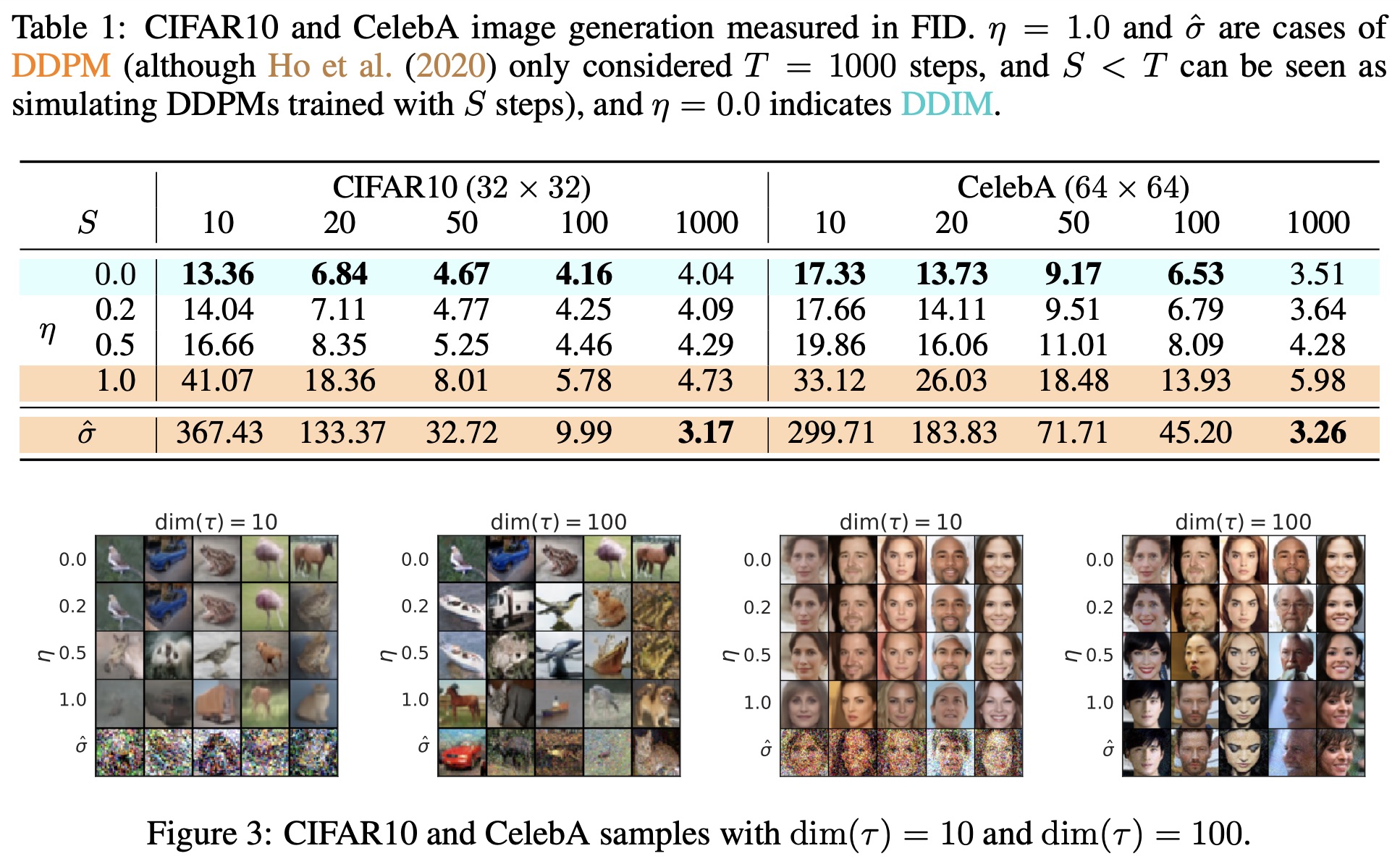DDIM's experimental results, showing that the smaller the noise, the better the generation quality after acceleration

The author's reference implementation is as follows:

GitHub: https://github.com/bojone/Keras-DDPM/blob/main/ddim.py

个人的实验结论是：

1. Perhaps counterintuitively, the smaller $\sigma_t$ is during generation, the relatively greater the noise and diversity of the final generated images tend to be;
2. The fewer diffusion steps $\dim(\boldsymbol{\tau})$ there are, the smoother the generated images become, and diversity also decreases somewhat;
3. Combining points 1 and 2, we find that when the number of diffusion steps $\dim(\boldsymbol{\tau})$ is reduced, one can appropriately shrink $\sigma_t$ to keep the quality of the generated images roughly unchanged, which is consistent with the experimental conclusions in the original DDIM paper;
4. When $\sigma_t$ is small, using a fixed Sinusoidal encoding to represent $t$ produces images with less noise than using a trainable Embedding layer;
5. When $\sigma_t$ is small, the original paper's U-Net architecture (found in ddpm2.py on GitHub) produces images with less noise than the U-Net architecture I devised myself (found in ddpm.py on GitHub);
6. That said, my personal impression is that, overall, the noise-free generation process performs worse than the noisy generation process, and when noise-free, the generation quality is more strongly affected by the model architecture.

Furthermore, when $\sigma_t=0$, DDIM is essentially a deterministic transformation that maps an arbitrary normal noise vector to an image, which is already almost identical to what a GAN does. So, analogous to GANs, we can interpolate between noise vectors and observe the corresponding generation results. But note that both DDPM and DDIM are quite sensitive to the noise distribution, so we cannot use linear interpolation — we need to use spherical interpolation instead. This is because, by the additivity of normal distributions, if $\boldsymbol{z}_1,\boldsymbol{z}_2\sim\mathcal{N}(\boldsymbol{0}, \boldsymbol{I})$, then $\lambda\boldsymbol{z}_1 + (1-\lambda)\boldsymbol{z}_2$ will generally no longer follow $\mathcal{N}(\boldsymbol{0}, \boldsymbol{I})$; we need to change it to

\begin{equation}\boldsymbol{z} = \boldsymbol{z}_1 \cos\frac{\lambda\pi}{2} + \boldsymbol{z}_2 \sin\frac{\lambda\pi}{2},\quad \lambda\in[0, 1]\end{equation}

Interpolation demo (from a model I trained myself):

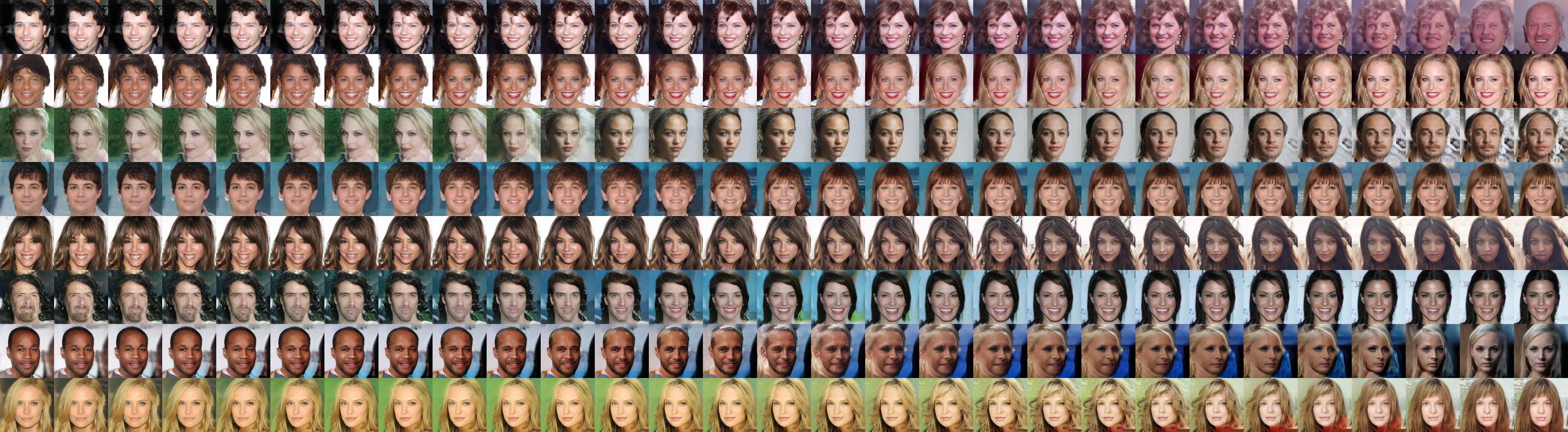Interpolated generation from DDIM random vectors

Finally, let's take a close look at the case $\sigma_t = 0$. In this situation, $\eqref{eq:sigma=0}$ can be equivalently rewritten as:

\begin{equation}\frac{\boldsymbol{x}_t}{\bar{\alpha}_t} - \frac{\boldsymbol{x}_{t-1}}{\bar{\alpha}_{t-1}} = \left(\frac{\bar{\beta}_t}{\bar{\alpha}_t} - \frac{\bar{\beta}_{t-1}}{\bar{\alpha}_{t-1}}\right) \boldsymbol{\epsilon}_{\boldsymbol{\theta}}(\boldsymbol{x}_t, t)\end{equation}

When $T$ is sufficiently large, or in other words $\alpha_t$ and $\alpha_{t-1}$ are sufficiently small, we can regard the above equation as the difference form of some ordinary differential equation. In particular, by introducing a virtual time parameter $s$, we obtain

\begin{equation}\frac{d}{ds}\left(\frac{\boldsymbol{x}(s)}{\bar{\alpha}(s)}\right) = \boldsymbol{\epsilon}_{\boldsymbol{\theta}}\left(\boldsymbol{x}(s), t(s)\right)\frac{d}{ds}\left(\frac{\bar{\beta}(s)}{\bar{\alpha}(s)}\right)\label{eq:ode}\end{equation}

Without loss of generality, assume $s\in[0,1]$, where $s=0$ corresponds to $t=0$ and $s=1$ corresponds to $t=T$. Note that the original DDIM paper directly uses $\frac{\bar{\beta}(s)}{\bar{\alpha}(s)}$ as the virtual time parameter, which in principle is not really appropriate, since its range is $[0,\infty)$ — an unbounded interval is not conducive to numerical solving.

So what we now need to do is, given $\boldsymbol{x}(1)\sim \mathcal{N}(\boldsymbol{0},\boldsymbol{I})$, solve for $\boldsymbol{x}(0)$. The iterative process of DDPM or DDIM corresponds to the Euler method for this ordinary differential equation. As is well known, the Euler method is relatively the slowest in terms of efficiency; if we want to speed up the solving process, we can use the Heun method, the Runge-Kutta method, and so on. In other words, once we identify the generation process with solving an ordinary differential equation, we can draw on numerical methods for ODEs to provide a much richer and more diverse set of tools for accelerating generation.

Let's take DDPM's default parameters $T=1000$, $\alpha_t = \sqrt{1 - \frac{0.02t}{T}}$ as an example and repeat the estimate we did in Generative Diffusion Models: A Chat (1): DDPM = Demolition + Construction

\begin{equation}\log \bar{\alpha}_t = \sum_{i=k}^t \log\alpha_k = \frac{1}{2} \sum_{k=1}^t \log\left(1 - \frac{0.02k}{T}\right) < \frac{1}{2} \sum_{k=1}^t \left(- \frac{0.02k}{T}\right) = -\frac{0.005t(t+1)}{T}\end{equation}

Since each $\alpha_k$ is very close to 1, the estimate above is in fact also a good approximation. And since our starting point in this post was $p(\boldsymbol{x}_t|\boldsymbol{x}_0)$, we should begin from $\bar{\alpha}_t$; based on the approximation above, we can simply take

\begin{equation}\bar{\alpha}_t = \exp\left(-\frac{0.005t^2}{T}\right) = \exp\left(-\frac{5t^2}{T^2}\right)\end{equation}

If we take $s=t/T$ as the parameter, then we get exactly $s\in[0,1]$, in which case $\bar{\alpha}(s)=e^{-5s^2}$. Substituting this into equation $\eqref{eq:ode}$ and simplifying gives

\begin{equation}\frac{d\boldsymbol{x}(s)}{ds} = 10s\left(\frac{\boldsymbol{\epsilon}_{\boldsymbol{\theta}}\left(\boldsymbol{x}(s), sT\right)}{\sqrt{1-e^{-10s^2}}} - \boldsymbol{x}(s)\right)\end{equation}

Alternatively, we can take $s=t^2/T^2$ as the parameter, in which case we also have $s\in[0,1]$, along with $\bar{\alpha}(s)=e^{-5s}$. Substituting these into equation $\eqref{eq:ode}$ and simplifying gives

\begin{equation}\frac{d\boldsymbol{x}(s)}{ds} = 5\left(\frac{\boldsymbol{\epsilon}_{\boldsymbol{\theta}}\left(\boldsymbol{x}(s), \sqrt{s}T\right)}{\sqrt{1-e^{-10s}}} - \boldsymbol{x}(s)\right)\end{equation}

Summary of this article

Continuing the derivation approach from the previous post on DDPM, this article introduces DDIM. It revisits the starting point of DDPM, removes the $p(\boldsymbol{x}_t|\boldsymbol{x}_{t-1})$ assumption made in the derivation, and thereby obtains a broader family of solutions along with a way to accelerate the generation process. Finally, this new family of solutions also allows us to connect the generation process with the solving of ordinary differential equations, so that we can further study the generation process using methods from ODE theory.