Variational Autoencoders (VI): An Attempt to Understand VAEs from a Geometric Perspective
A while back my company organized an internal tech talk, and when it was my turn, everyone asked me to talk about VAEs. Since I'd already written a series of posts on variational autoencoders, this shouldn't have been too hard for me, so I agreed to do it. But on second thought, I realized it was actually a tricky task: how should I present it?
Regarding VAEs, I have two relatively systematic introductions from before: Variational Autoencoders (I): So That's What It Is and Variational Autoencoders (II): Starting from a Bayesian Viewpoint. The latter is a purely probabilistic derivation, which isn't of much use to people who aren't doing theoretical research, and isn't necessarily easy to follow. The former, while a bit more accessible, isn't quite right either, because it approaches things from the angle of generative models, and doesn't really clarify "why we need VAEs" at all (to put it bluntly, VAEs can give us generative models, but VAEs aren't necessarily for generative models). Overall its style isn't especially friendly either.
After some thought, I realized that for most readers who don't yet understand VAEs but want to use them, what they probably want is just a rough grasp of the form of a VAE, along with answers to questions like "What does a VAE actually do?", "How is a VAE different from an AE?", and "In what scenarios do we need a VAE?" Neither of the two articles above satisfies this kind of need very well. So I tried to construct a geometric picture of VAEs, attempting to describe their key properties from a geometric angle, which I'd like to share with you here.
Autoencoders
Let's start with the autoencoder (AE). The original motivation for autoencoders was dimensionality reduction: suppose the raw features $x$ have too high a dimension, so we want an encoder $E$ to encode them into a low-dimensional feature vector $z=E(x)$. The principle behind the encoding is to preserve as much of the original information as possible, so we also train a decoder $D$, hoping to reconstruct the original information from $z$, i.e., $x\approx D(E(x))$. The optimization objective is generally
\begin{equation}E,D = \mathop{\text{argmin}}_{E,D}\mathbb{E}_{x\sim \mathcal{D}}\big[\Vert x - D(E(x))\Vert^2\big]\end{equation}
The corresponding diagram is as follows:
 Diagram of an autoencoder
The encoding space
If every sample can be reconstructed well, then we can treat $z$ as an equivalent representation of $x$—that is, studying $z$ thoroughly is as good as studying $x$ thoroughly. Now, if we encode every $x$ into its corresponding feature vector $z$, we naturally care about a question: what does the space covered by all these $z$ "look like"?
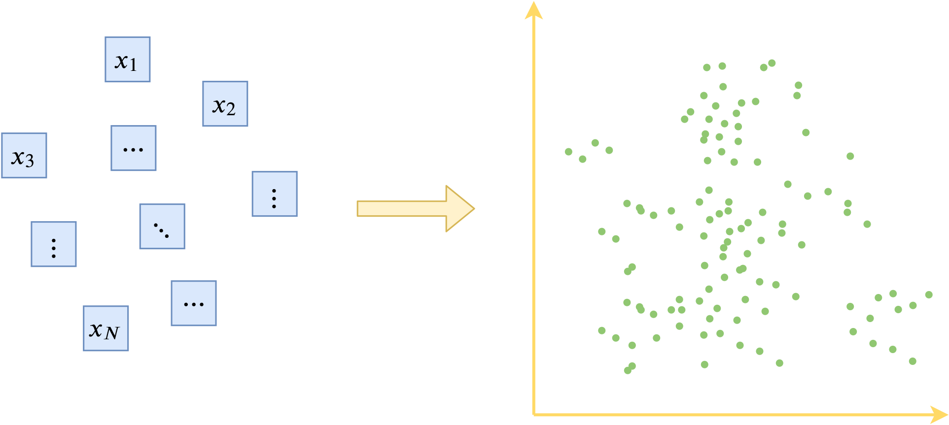 After passing through the autoencoder, an original sample corresponds to a point in the encoding space
Why should we care about this question? Because there are many different ways to encode, and the feature vectors produced by different encoding schemes can be better or worse—and from "what the encoding space looks like," we can roughly judge how good the feature vectors are. For instance, consider the following simulated shapes of four different distributions of encoding vectors:
 Four simulated shapes of the encoding space, representing no particular pattern, a line, a ring, and a circle respectively
The vectors in the first figure have no particular shape and are fairly scattered, suggesting the encoding space isn't especially well-organized. In the second figure, the vectors are concentrated on a line, which suggests there's actually redundancy across the dimensions of the encoding vector. The third figure is a ring, meaning there's no real sample corresponding to the region near the center. The fourth figure is a disk, indicating it covers a continuous region of space fairly neatly. Comparing these four figures, we'd consider the shape in the last one to be the most ideal: neat, non-redundant, and continuous. This means that once we've learned from part of the samples, it's easy to generalize to new, unseen samples, because we know the encoding space is neat and continuous—so we know that the "gaps" between the encoding vectors of the training samples (the blank areas between two points in the figure) actually also correspond to real, as-yet-unseen samples. So if we handle the known part well, chances are we've also handled the unknown part well.
From points to regions
Broadly speaking, we care about the following questions regarding the encoding space:
1. What kind of region do all the encoding vectors cover?
2. Are there unknown real samples corresponding to the vectors in the blank areas?
3. Are there any "outlier" vectors that have strayed from the crowd?
4. Is there a way to make the encoding space more regular/neat?
Since ordinary autoencoders come with no particular constraints, it's hard to answer the questions above with them. This is where the variational autoencoder comes in. From the encoding perspective, its goals are: 1. Make the encoding space more regular; 2. Make the encoding vectors more compact. To achieve this, the variational autoencoder first introduces a posterior distribution $p(z|x)$.
For readers who'd rather not dig into the language of probability, how should we understand the posterior distribution $p(z|x)$? Intuitively, we can think of the posterior distribution as an "ellipse." Originally, each sample corresponded to an encoding vector, i.e., a single point in the encoding space; after introducing the posterior distribution, each sample $x$ now corresponds instead to an "ellipse." We said earlier that we want the encoding vectors to be more "compact," but in theory, no matter how many "points" you use, they can never fully cover a "region"—but if you cover a "region" with "regions," then it becomes easy to cover the target. This is one of the main changes made by the variational autoencoder.
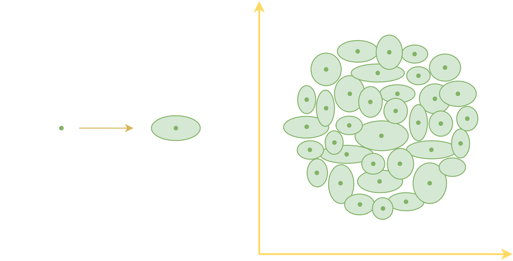 Each sample's encoding goes from a point to a region (an ellipse), so the encoding space, originally covered by points, is now covered by regions
Readers might ask: why does it have to be an ellipse? Could it be a rectangle or some other shape? Going back to the language of probability, an ellipse corresponds to "assuming a Gaussian distribution $p(z|x)$ with independent components." From a probabilistic standpoint, Gaussian distributions are relatively easy to work with, so we use Gaussian distributions—which correspond to ellipses. Other shapes correspond to other distributions; for example, a rectangle could correspond to a uniform distribution, but that turns out to be troublesome later on when computing the KL divergence, so it's generally not used.
Sampling and reconstruction
Now every sample $x$ corresponds to an "ellipse," and determining an "ellipse" requires two pieces of information: the center of the ellipse and the lengths of its axes, each of which forms a vector, and both depend on the sample $x$, which we denote as $\mu(x),\sigma(x)$. Since the entire ellipse now corresponds to sample $x$, we require that any point inside the ellipse be able to reconstruct $x$. So the training objective is:
\begin{equation}\mu,\sigma,D = \mathop{\text{argmin}}_{\mu,\sigma,D}\mathbb{E}_{x\sim \mathcal{D}}\big[\Vert x - D(\mu(x) + \varepsilon\otimes \sigma(x))\Vert^2\big],\quad \varepsilon\sim \mathcal{N}(0, 1)\end{equation}
where $\mathcal{D}$ is the training data, and $\mathcal{N}(0, 1)$ is the standard normal distribution, which we can think of as a unit circle. That is, we first sample $\varepsilon$ from inside the unit circle, then apply a shift-and-scale transformation $\mu(x) + \varepsilon\otimes \sigma(x)$ to turn it into a point inside the ellipse "centered at $\mu(x)$ with axis lengths $\sigma(x)$." This process is what's known as "reparameterization."
Here, $\mu(x)$ actually corresponds to the encoder $E(x)$ in the autoencoder, and $\sigma(x)$ corresponds to the range over which it can generalize.
Regularizing the space
Finally, the "ellipse" can "make the encoding vectors more compact," but it still can't "make the encoding space more regular." Now we want the encoding vectors to satisfy a standard normal distribution (which we can think of as a unit circle), i.e., we want the union of all the ellipses to form a single unit circle.
To this end, we want every ellipse to move closer to the unit circle, whose center is 0 and radius is 1. So a basic idea is to introduce a regularization term:
\begin{equation}\mathbb{E}_{x\sim \mathcal{D}}\big[\Vert \mu(x) - 0\Vert^2 + \Vert \sigma(x) - 1\Vert^2\big]\end{equation}
In fact, combining these two loss terms already gets us very close to the standard variational autoencoder. The standard VAE uses a somewhat more complex regularization term that serves a similar function:
\begin{equation}\mathbb{E}_{x\sim \mathcal{D}}\left[\sum_{i=1}^d \frac{1}{2}\Big(\mu_{i}^2(x) + \sigma_{i}^2(x) - \log \sigma_{i}^2(x) - 1\Big)\right]\end{equation}
This regularization term comes from the KL divergence between two Gaussian distributions, so it's usually called the "KL divergence term."
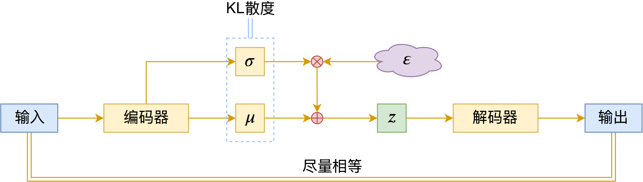 Diagram of a variational autoencoder
Combining the two objectives gives us the final variational autoencoder:
\begin{equation}\Vert x - D(\mu(x) + \varepsilon\otimes \sigma(x))\Vert^2 + \sum_{i=1}^d \frac{1}{2}\Big(\mu_{i}^2(x) + \sigma_{i}^2(x) - \log \sigma_{i}^2(x) - 1\Big), \quad \varepsilon\sim \mathcal{N}(0, 1)\end{equation}
Summary
This article introduced an understanding of the variational autoencoder (VAE) from the angle of a geometric analogy. Under this view, the goal of the VAE is to make the encoding vectors more compact, and to regularize the encoding distribution so that it becomes a standard normal distribution (a unit circle).
In doing so, the VAE achieves two effects: 1. By randomly sampling a vector from the standard Gaussian distribution (the unit circle), the decoder can produce a realistic sample—that is, it realizes a generative model; 2. Because of the compactness of the encoding space, together with the noise injected into the encoding vectors during training, the individual components of the encoding vector become disentangled to some degree, and the encoding vector acquires certain linear-arithmetic properties.
The geometric perspective lets us quickly grasp the key properties of the variational autoencoder and lowers the barrier to entry, though it does come with a certain lack of rigor. If there's anything inappropriate here, I hope readers will understand and point it out.
Translated automatically with claude-sonnet-5; all equations are reproduced verbatim from the source. Copyright remains with the original author.