Google's New Work Attempts to "Resurrect" RNNs: Can RNNs Shine Again?

Google新作试图“复活”RNN：RNN能否再次辉煌？ 苏剑林 · 2023-03-28 · Machine Learning language model RNN generative model attention

LLMs like ChatGPT are currently sweeping the world. Some readers have noticed that almost all LLMs still use the original Multi-Head Scaled-Dot Attention, while the large body of recent efficient-attention work such as linear attention and FLASH has not been widely adopted. Is it because these variants simply perform worse, or is efficiency just not a real concern to begin with? I've actually analyzed this before in Linear Transformers Are Probably Not the Model You're Waiting For: standard attention only exhibits quadratic complexity once the sequence length clearly exceeds the hidden size; before that point it remains close to linear, and it's actually faster than many "efficient" alternatives. Since models like GPT-3 use hidden sizes in the tens of thousands, this means that unless your LLM is meant to generate text with tens of thousands of tokens, adopting an efficient variant is unnecessary — in many cases you don't even gain speed, and performance drops instead.

So when we genuinely do need to handle sequences of tens or even hundreds of thousands of tokens, what model should we use? Recently, a Google paper, Resurrecting Recurrent Neural Networks for Long Sequences, re-optimized the RNN and specifically highlighted its advantages in handling extremely long sequences. So, can RNNs shine again? more

Linearization

The RNN proposed in the paper is called the LRU (Linear Recurrent Unit) — a minimalist linear RNN that can be run both in parallel and sequentially, making it efficient for both training and inference. LRU shares a lot in common with works like SSM (Structured State Model) and RWKV. In fact, the starting point of LRU was the observation that SSMs perform very well on LRA, which motivated the search for a way to make a vanilla RNN perform equally well on LRA — and the result was LRU. Unfortunately, the original paper only ran experiments on LRA (Long Range Arena, a benchmark testing long-range dependency modeling); at the end of this post I'll supplement this with some of my own experimental results on language modeling.

The original paper's exposition starts from SSMs and spends considerable space describing the connection between LRU and SSMs. In this post, we'll skip over that connection and instead derive and introduce LRU directly as a standalone RNN model. As we know, the simplest RNN can be written as

\begin{equation}x_t = f(Ax_{t-1} + u_t)\end{equation}

where $x_t,u_t\in\mathbb{R}^d,A\in\mathbb{R}^{d\times d}$, and $f$ is the activation function. In general there would also be a projection matrix before $u_t$ and after $x_t$, but here we focus on the recurrence itself, so we won't write those explicitly.

Conventional wisdom holds that the activation function must be nonlinear — common choices include $\text{sigmoid},\tanh,\text{relu}$, and in particular some work has shown that a single-layer RNN with $\text{sigmoid}$ or $\tanh$ activation is Turing complete, which reinforces the belief that a nonlinear activation is essential. However, in deep learning, experiments are the sole criterion for truth, and the authors found that when replacing Transformer self-attention with an RNN, a linear RNN actually performs best:

Across the various LRA tasks, the linear RNN is actually the best

This is a surprisingly good piece of news. "Surprising" because it may overturn some readers' assumptions about a model's need for nonlinearity; though of course, some readers might not be so surprised, since works like MetaFormer have already shown that, thanks to the power of the FFN layer, the token-mixing layer (e.g. self-attention) can have very weak nonlinearity — even a pooling layer works. As for "good news," that's because a linear RNN admits a parallel implementation, which makes it far faster to compute than a nonlinear RNN.

So, the authors carried out a series of investigations centered on linear RNNs.

Diagonalization

Removing the activation function, the RNN simplifies once again to

\begin{equation}x_t = Ax_{t-1} + u_t\label{eq:lr}\end{equation}

Iterating this repeatedly gives

\begin{equation}x_0 = u_0\\ x_1 = Au_0 + u_1\\ x_2 = A^2 u_0 + Au_1 + u_2\\ \vdots \\ x_t = \sum_{k=0}^t A^{t-k}u_k\label{eq:lr-e}\end{equation}

As we can see, most of the computation is concentrated in computing powers of the matrix $A$. This naturally brings to mind matrix diagonalization, an efficient way to compute matrix powers — except that a general matrix isn't necessarily diagonalizable over the reals. What can we do then? Let's broaden our horizons a bit: if it doesn't work over the reals, let's go to the complex domain! Almost every matrix can be diagonalized over the complex numbers, which means $A$ can always be written as

\begin{equation}A = P\Lambda P^{-1}\quad\Rightarrow\quad A^n = P\Lambda^n P^{-1}\end{equation}

where $P,\Lambda\in\mathbb{C}^{d\times d}$, and $\Lambda$ is a diagonal matrix of eigenvalues. Substituting this into $\eqref{eq:lr-e}$, we get:

\begin{equation}x_t = \sum_{k=0}^t P\Lambda^{t-k}P^{-1}u_k = P\left(\sum_{k=0}^t \Lambda^{t-k}(P^{-1}u_k)\right)\end{equation}

As mentioned earlier, in general there's also a projection matrix before $u_t$ and after $x_t$; as long as we stipulate that both of these projection matrices are complex-valued, then in principle $P$ and $P^{-1}$ can both be absorbed into their respective projections. This means that, as long as everything is computed over the complex domain, replacing the general matrix $A$ in the linear RNN with the diagonal matrix $\Lambda$ incurs no loss of model capacity whatsoever! So we only need to consider the following minimalist RNN:

\begin{equation}x_t = \Lambda x_{t-1} + u_t\quad\Rightarrow\quad x_t = \sum_{k=0}^t \Lambda^{t-k}u_k\label{eq:lr-x}\end{equation}

Parametrization

The advantage of a diagonal matrix is that all operations become element-wise, so the computation along each dimension can be fully parallelized; it also means that analyzing a single dimension is equivalent to analyzing all of them, so the model analysis can be carried out entirely in one-dimensional space. Let's set $\Lambda=\text{diag}(\lambda_1,\lambda_2,\cdots,\lambda_d)$, and let $\lambda$ denote one entry of $\lambda_1,\lambda_2,\cdots,\lambda_d$; when there's no risk of confusion, we'll also let $x_t$ and $u_t$ denote the corresponding components of $\lambda$, so that $\eqref{eq:lr-x}$ simplifies to a scalar computation:

\begin{equation}x_t = \lambda x_{t-1} + u_t\quad\Rightarrow\quad x_t = \sum_{k=0}^t \lambda^{t-k}u_k\label{eq:lr-xx}\end{equation}

Note that $\lambda$ is complex, so we can write $\lambda = re^{i\theta}$, where $r \geq 0, \theta\in[0, 2\pi)$ are both real numbers:

\begin{equation}x_t = \sum_{k=0}^t r^{t-k}e^{i(t-k)\theta}u_k\label{eq:lr-e-r-theta}\end{equation}

During summation, all the $t-k$ terms are non-negative, so we need $r \leq 1$ — otherwise the weight on historical terms would grow without bound, which conflicts with our intuition (intuitively, dependence on history should weaken over time) and also risks exploding gradients. On the other hand, if $r \ll 1$, there's a risk of vanishing gradients. This places two requirements on $r$: 1) we must guarantee $r\in[0,1]$; 2) at initialization, $r$ should be as close to 1 as possible.

To achieve this, let's first set $r = e^{-\nu}$, so $r\in[0,1]$ requires $\nu\geq 0$; we then further set $\nu=e^{\nu^{\log}}$, giving us $\nu^{\log}\in\mathbb{R}$, turning this into unconstrained optimization. Here $\nu^{\log}$ is just the notation for another variable, not a special operation. And since $\nu$ has been parametrized as $e^{\nu^{\log}}$, for consistency we'll also parametrize $\theta$ as $e^{\theta^{\log}}$.

Readers might ask: there are many ways to enforce the constraint $r\in[0,1]$ — why go to all this trouble? Wouldn't a simple sigmoid do? First, once $r$ is parametrized as $e^{-\nu}$, the power operation can be merged with $\theta$, i.e. $r^k e^{ik\theta}=e^{k(-\nu+i\theta)}$, which is convenient both for implementation and computation. Second, since $\nu\geq 0$, the simplest smooth function that maps any real number to a non-negative number is likely the exponential function, which naturally leads to $\nu=e^{\nu^{\log}}$. The activation used in SSMs, $\text{relu}$, i.e. directly $r=e^{-\max(\nu,0)}$, has a saturation region that may hinder optimization.

Initialization

Next let's consider the initialization problem. Going back to the original form $\eqref{eq:lr}$, for a real matrix of shape $d\times d$, standard Glorot initialization draws entries from a normal or uniform distribution with mean 0 and variance $1/d$ (see Understanding Model Parameter Initialization Strategies from a Geometric Perspective). It can be shown theoretically or experimentally that the eigenvalues of a matrix initialized this way are roughly uniformly distributed over the unit disk in the complex plane:

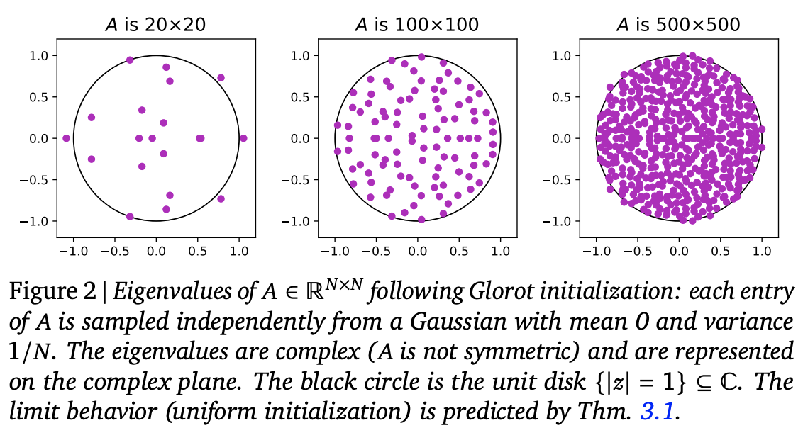The eigenvalues of a Glorot-initialized matrix are uniformly distributed within the unit disk

This suggests that a natural standard initialization for $\Lambda$ is to uniformly sample points within the unit disk in the complex plane. Switching from Cartesian to polar coordinates, we have $dxdy=rdrd\theta=\frac{1}{2}d(r^2)d\theta$, which tells us that to achieve uniform sampling within the unit disk, we simply need $\theta\sim U[0,2\pi]$ and $r^2\sim U[0,1]$.

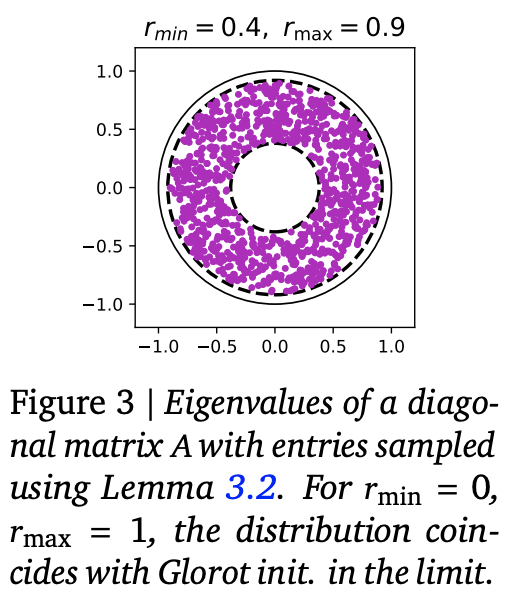Switching to an annulus initialization gives better performance on most tasks

However, as mentioned earlier, to guard as much as possible against vanishing gradients, we want $r$ to be as close to 1 as possible at initialization, so the improved approach is to sample uniformly within an annulus near $r\in[r_{\min},r_{\max}]$, changing the sampling scheme to $\theta\sim U[0,2\pi]$ and $r^2\sim U[r_{\min}^2,r_{\max}^2]$. The original paper's experimental results show that $r_{\min}=0.9,r_{\max}=0.999$ works well for most experiments.

There's a subtlety here: since $r$ is initialized close to 1, and at the initial stage $u_t$ is roughly i.i.d., equation $\eqref{eq:lr-e-r-theta}$ approximates a sum (rather than an average) of several terms whose magnitude is roughly preserved — which risks explosion. To analyze this, let's first write

\begin{equation}|x_t|^2 = x_t x_t^* = \sum_{k=0}^t\sum_{l=0}^t r^{(t-k)+(t-l)}e^{i[(t-k)-(t-l)]\theta}u_k u_l^*\end{equation}

Here $*$ denotes complex conjugation and $|\cdot|$ denotes the modulus of a complex number. Taking expectations on both sides, and assuming $u_k,u_l$ are i.i.d. with mean zero, when $k\neq l$ we have $\mathbb{E}[u_k u_l^*]=\mathbb{E}[u_k]\mathbb{E}[u_l^*]=0$, so only the terms with $k=l$ survive, giving:

\begin{equation}\mathbb{E}[|x_t|^2] = \sum_{k=0}^t r^{2(t-k)}\mathbb{E}[u_k u_k^*] = \mathbb{E}[|u_k|^2]\sum_{k=0}^t r^{2(t-k)} = \frac{(1 - r^{2(t+1)})\mathbb{E}[|u_k|^2]}{1-r^2}\end{equation}

Since $r \in (0, 1)$, when $t$ is sufficiently large, $r^{2(t+1)}\to 0$. In other words, when $t$ is fairly large, on average the ratio between the magnitude of $x_t$ and that of $u_k$ is $\frac{1}{\sqrt{1-r^2}}$; when $r$ is very close to 1, this ratio becomes large, meaning that the sequence gets amplified substantially after passing through the RNN, which is bad for training stability. To address this, the authors introduced a simple trick: an additional element-wise parameter $\gamma$, initialized to $\sqrt{1-r^2}$, changing equation $\eqref{eq:lr-xx}$ to:

\begin{equation}x_t = \lambda x_{t-1} + \gamma u_t\quad\Rightarrow\quad x_t = \gamma\sum_{k=0}^t \lambda^{t-k} u_k\label{eq:lr-xxx}\end{equation}

This way, at least at the start, the model's output magnitude is stabilized, and the rest can be left to the model to learn. Putting all of this together gives us the LRU (Linear Recurrent Unit) model proposed in the original paper, as shown below:

Diagram of the LRU model

Related Variants

Here we introduce two variants related to LRU.

SLRU

LRU starts from simplifying a general linear RNN model $\eqref{eq:lr}$, and in order to theoretically match the expressive power of a general matrix, it has no choice but to introduce complex projection matrices and a complex diagonal matrix of eigenvalues $\Lambda$. If we don't care about matching the power of a general matrix, and are purely concerned with the decaying effect provided by $r$, we can simplify LRU even further by assuming that both the projection matrices and the diagonal eigenvalue matrix are real — we call this simplified version SLRU (Simpler Linear Recurrent Unit).

The original paper doesn't study SLRU, but I feel it aligns better with our intuition (mainly because changes in phase $\theta$ are less intuitive to reason about), so I've included experiments with SLRU later in this post.

RWKV

Speaking of RNNs, some readers may have heard of the recently somewhat famous RWKV, which can be viewed as a combination of SLRU/Hydra Attention and a GLU (Gated Linear Unit). The RNN part of RWKV is:

\begin{equation}x_t = \sigma(r_t) \times\frac{y_t + (\gamma \lambda - 1)e^{k_t}v_t}{z_t + (\gamma \lambda - 1)e^{k_t}},\quad\begin{aligned}y_t =&\, \lambda y_{t-1} + e^{k_t}v_t \\ z_t =&\, \lambda z_{t-1} + e^{k_t}\end{aligned}\end{equation}

As you can see, the recurrent part consists of two SLRUs; RWKV's distinguishing feature is that the results of the two SLRUs are divided by each other, achieving a normalizing effect, so it doesn't need the gamma trick used in LRU. Additionally, perhaps to match the parameter count of self-attention, or to further boost performance, after normalization RWKV also multiplies in an additional gate $\sigma(r_t)$. Although the authors have already validated RWKV's effectiveness on LM tasks, a controlled comparison against common models seems to be missing, and this post will supplement that.

Note: "RWKV" here refers specifically to the RNN module responsible for token mixing, not the full model given by the authors (i.e., it excludes their Channel-Mix layer, time shift, etc.).

Implementation

In this section we discuss how to implement LRU. The appendix of the original paper provides reference code in Jax; here I'll also provide a Keras version:

GitHub: https://github.com/bojone/rnn

There are two technical challenges to implementing LRU: handling complex numbers and parallelization.

Handling Complex Numbers

LRU's projection matrices and eigenvalues are complex-valued. The Jax code given by the authors uses complex matrices directly, but switching to Keras means we can't reuse the existing Dense layer, which is a bit of a shame. In fact, from $(B+iC)u=Bu + iCu$ we can see that a complex projection matrix is just a projection with double the output dimension, so for the projection part we don't need complex matrices at all — we can just use a Dense layer with twice the number of units.

Next is the $e^{i(t-k)}u_k$ part, which can either be expanded directly into pure real-valued operations, or computed directly in complex arithmetic following the formula. If expanded into real operations, its form turns out to be identical to RoPE, so when I first saw LRU I got quite excited, thinking "isn't this just 'RoPE is all you need'?" That said, after comparing speeds, I found that implementing it directly with complex arithmetic following the formula is actually slightly faster, so I'd recommend using the complex version.

Finally, there's the issue of projecting the complex output back into a real matrix. From $\Re[(B+iC)(x+iy)]=Bx-Cy=[B,-C][x,y]^{\top}$, this means we simply need to concatenate the real and imaginary parts and then feed them through a Dense layer.

Parallelization

If we implement the RNN sequentially, strictly following the recurrence formula, training will be extremely slow (prediction is fine since autoregressive generation is inherently sequential anyway). As mentioned earlier, an important property of linear RNNs is that they admit a parallel algorithm, which can greatly speed up training.

In fact, we can rewrite $\eqref{eq:lr-xx}$ as

\begin{equation}x_t = \lambda^t \sum_{k=0}^t \lambda^{-k} u_k\end{equation}

This already reveals a fast algorithm: multiply each $u_k$ by $\lambda^{-k}$, which is element-wise and parallelizable; then the $\sum\limits_{k=0}^t$ step is actually just a cumsum operation, which is implemented efficiently in most frameworks; finally, multiply each result of cumsum by the corresponding $\lambda^t$, which is again element-wise and parallelizable. However, since $|\lambda| < 1$, when $k$ is large, $\lambda^{-k}$ will almost certainly explode — forget fp16, even FP32 or FP64 may not be enough to hold up for long sequences. So while this scheme looks elegantly simple, and is theoretically sound, it's of little practical value.

The key to parallel acceleration is noticing the decomposition ($T > t$)

\begin{equation}\begin{aligned} x_T =&\, \sum_{k=0}^T \lambda^{T-k} u_k \\ =&\, \sum_{k=0}^t \lambda^{T-k} u_k + \sum_{k=t+1}^T \lambda^{T-k} u_k \\ =&\, \lambda^{T-t}\sum_{k=0}^t \lambda^{t-k} u_k + \sum_{k=t+1}^T \lambda^{T-k} u_k \\ \end{aligned}\end{equation}

This decomposition tells us that computing $\eqref{eq:lr-xx}$ over the whole sequence is equivalent to splitting the sequence into two halves, computing $\eqref{eq:lr-xx}$ on each half independently, and then adding the last result of the first half — appropriately weighted — to every position in the second half, as shown on the left below:

Parallel recursive decomposition of a linear RNNFull expansion of the linear RNN's recursive decomposition

The key here is that "splitting into two halves and computing $\eqref{eq:lr-xx}$ separately" — these two halves can be computed in parallel! Recursing on this, we turn what was originally a loop of $\mathcal{O}(L)$ steps into $\mathcal{O}(\log L)$ steps, greatly speeding up training, as shown on the right above.

In fact, this is precisely the "Upper/Lower" parallel algorithm for the prefix sum problem; you can find the implementation details in the code linked above. Since TensorFlow 1.x doesn't support writing recursion directly, I implemented it bottom-up using tf.while_loop or for; when training, this can only barely approach the speed of self-attention. In fact, if the loop part were rewritten as a CUDA kernel, it should be possible to exceed the speed of self-attention (unfortunately, that's beyond my skills). The author of RWKV only wrote RWKV's RNN formulation as a CUDA kernel, without considering parallelization, and even that alone was already enough to rival the speed of self-attention.

There's also an "Odd/Even" parallel algorithm for prefix sum, which is theoretically somewhat more computationally efficient, but has a more complex structure. If implemented in TensorFlow, it involves more loop steps as well as more reshape and concat operations, and its actual efficiency may not necessarily beat the "Upper/Lower" parallel algorithm — so I didn't implement it (mainly because TensorFlow 1.x doesn't support recursion; if written with recursion, it wouldn't be too complicated).

Experimental Results

In this section, we'll present the original paper's experimental results on LRA, along with my own experimental results on language modeling (LM) tasks.

In the original paper, the authors mainly combine theory and experiment to demonstrate, step by step, how to optimize a plain RNN until it achieves near-SOTA performance on LRA. This process of analysis and refinement is genuinely engaging and worth savoring repeatedly. However, since all the paper's experiments are conducted repeatedly on LRA, there isn't much extra to showcase here beyond Table 8 from the paper:

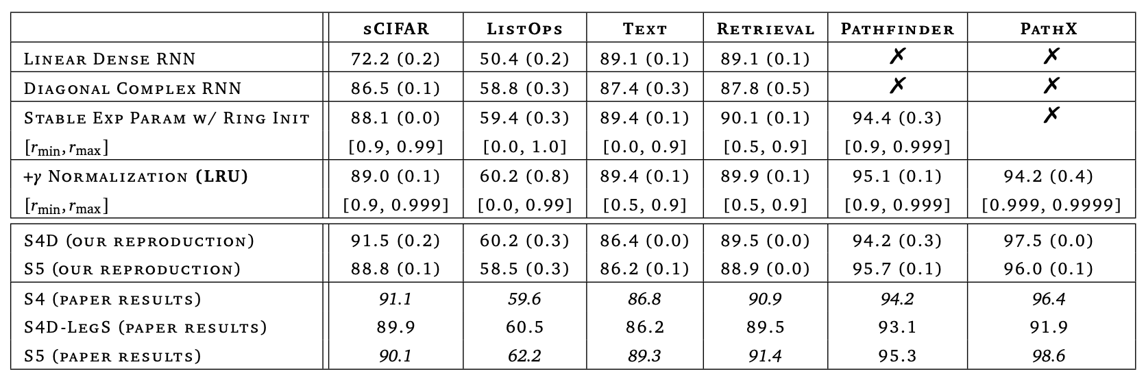Summary of experimental results from the LRU paper

Readers of this blog are likely more interested in its performance on NLP tasks, especially the currently hot LM tasks — unfortunately the original paper doesn't cover this, so I ran some comparison experiments myself for reference. The models compared include GAU (same as GAU-α), SA (same as RoFormerV2), LRU, SLRU, and RWKV, where LRU, SLRU, and RWKV are simply RoFormerV2 with self-attention replaced by LRU, SLRU, or RWKV modules with similar parameter counts and compute cost. All models are base-sized, with roughly 100M parameters — which counts as a small model these days. All models use DeepNorm initialization, Tiger as the optimizer, and all other hyperparameters are kept identical, giving a fairly well-controlled comparison.

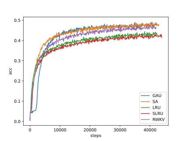
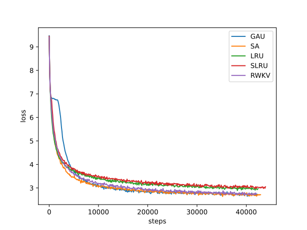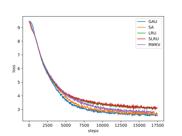
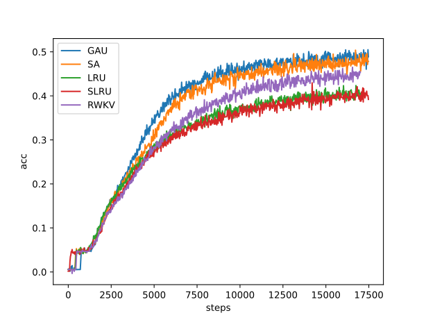
Loss curves for training length 128Accuracy curves for training length 128Loss curves for training length 512Accuracy curves for training length 512

As we can see, ranked by performance, the ordering should be

$$\text{GAU} > \text{SA} > \text{RWKV} > \text{LRU} > \text{SLRU}$$

From these experimental results we can draw the following conclusions:

1. LRU outperforms SLRU, showing that introducing complex projection matrices and complex eigenvalues genuinely helps — though it comes at some cost in computational efficiency (even when the parameter count is held constant);
2. As sequence length increases, the attention-based models (GAU, SA) get better, while the RNN-based models (LRU, SLRU, RWKV) get worse — this is a fundamental difference between the two families, presumably because an RNN's long-range memory capacity is bottlenecked by its hidden size;
3. RWKV is indeed likely the best RNN model available right now, but there's still a clear gap compared to attention-based models (GAU, SA);
4. Following from point 2, for the RNN family to catch up with the attention family, it would probably need a larger hidden size — so on LM tasks, RNNs may only show their advantage at a bigger scale;
5. Combining points 1 and 3: could the next improved RNN be a complex-valued version of RWKV?

There are also a few practical lessons from running these experiments. Since GAU is single-headed, in long-sequence, large-scale settings its computational efficiency is noticeably better than SA, and its performance is also better than SA — so GAU is probably the best choice for language models across a fairly wide range of settings. Off the top of my head, I'd recommend GAU as the default choice for models under ten billion parameters and sequence lengths under 5000. That said, it's undeniable that RNN-family models of the same scale have better inference efficiency (both the compute and cache size per recurrence step are constant), and their training efficiency is on par with attention-based models — so once scaled up, RNNs should still have a chance to compete with attention-based models.

It's worth pointing out that although RWKV performs well overall, there is still a gap compared to GAU and SA, so under a fair comparison, RWKV isn't quite as flawless as legend has it. In fact, the RWKV author's own implementation contains a series of tricks that are said to help improve LM performance but are quite obscure (according to the author, these tricks are the real "essence" of the method) — you'd only discover them by reading the author's source code, and I did not incorporate them into my experiments. It's entirely possible these tricks help train a better LM in practice, but my goal here was to run a fair controlled comparison rather than actually train a production LM; once you start introducing these tricks, there are too many variables, and given my limited compute, I couldn't test all of them systematically.

Of course, all the conclusions above are drawn only from "small" models at the 100M-parameter scale. I'm still experimenting with larger scales, and can't yet offer conclusions there.

Conclusion

This post introduced one of Google's attempts to "resurrect" the RNN, building from the ground up an efficient RNN model that achieves near-SOTA performance on LRA. Beyond the original paper's LRA experiments, this post also presented my own experimental results on language modeling, including comparisons against RWKV and related models. Overall, the optimized RNN model is not inferior to attention-based models in training efficiency, and offers better inference performance, but there is still a certain gap compared to attention-based models in language modeling performance — perhaps the model needs to be scaled up further before the advantages of RNNs become fully apparent.