Tiger: An Optimizer That's "Stingy" to the Extreme

Tiger：一个“抠”到极致的优化器 苏剑林 · 2023-03-07 · Machine Learning model optimization optimizer

I've spent the past while experimenting with the Lion optimizer introduced in Google's Newly Discovered Optimizer Lion: A "Training Lion" with Both Efficiency and Effectiveness. What made Lion so interesting to me is that it coincides with some of my earlier ideas about an "ideal optimizer" — ideas I had failed to make work well at the time, but which Lion managed to pull off.

Compared to standard Lion, what interests me more is the special case where $\beta_1=\beta_2$, which I call "Tiger" here. Tiger only uses momentum to construct the update, and according to the conclusions in Gradient Accumulation Hidden Inside Momentum: Fewer Updates, Better Results?, in this case we can implement gradient accumulation "invisibly," without introducing an extra set of parameters! This means that whenever we need gradient accumulation, Tiger has already reached the theoretically optimal solution in terms of GPU memory usage — which is also where the name "Tiger" comes from (Tight-fisted Optimizer, an optimizer too stingy to spend even a little extra memory).

In addition, Tiger incorporates some of our hyperparameter-tuning experience, and proposes a simple strategy for preventing NaNs in the model (especially under mixed-precision training). Our preliminary experiments show that these changes make Tiger friendlier for training models — especially large models. more

Basic Form

Tiger's update rule is

\begin{equation}\text{Tiger}:=\left\{\begin{aligned} &\boldsymbol{m}_t = \beta \boldsymbol{m}_{t-1} + \left(1 - \beta\right) \boldsymbol{g}_t \\ &\boldsymbol{\theta}_t = \boldsymbol{\theta}_{t-1} - \eta_t \left[\text{sign}(\boldsymbol{m}_t) \color{skyblue}{ + \lambda_t \boldsymbol{\theta}_{t-1}}\right] \\ \end{aligned}\right.\end{equation}

Compared to Lion, it simply fixes the parameter $\beta_1 = \beta_2 = \beta$; compared to SignSGD, it adds momentum and weight decay.

Reference implementation:

Tiger: https://github.com/bojone/tiger

The table below compares the update rules of Tiger, Lion, and AdamW:

$$\begin{array}{c|c|c} \hline \text{Tiger} & \text{Lion} & \text{AdamW} \\ \hline {\begin{aligned} &\boldsymbol{m}_t = \beta \boldsymbol{m}_{t-1} + \left(1 - \beta\right) \boldsymbol{g}_t \\ &\boldsymbol{\theta}_t = \boldsymbol{\theta}_{t-1} - \eta_t \left[\text{sign}(\boldsymbol{m}_t) \color{skyblue}{ + \lambda_t \boldsymbol{\theta}_{t-1}}\right] \\ \end{aligned}} & {\begin{aligned} &\boldsymbol{u}_t = \text{sign}\big(\beta_1 \boldsymbol{m}_{t-1} + \left(1 - \beta_1\right) \boldsymbol{g}_t\big) \\ &\boldsymbol{\theta}_t = \boldsymbol{\theta}_{t-1} - \eta_t (\boldsymbol{u}_t \color{skyblue}{ + \lambda_t \boldsymbol{\theta}_{t-1}}) \\ &\boldsymbol{m}_t = \beta_2 \boldsymbol{m}_{t-1} + \left(1 - \beta_2\right) \boldsymbol{g}_t \end{aligned}} & {\begin{aligned} &\boldsymbol{m}_t = \beta_1 \boldsymbol{m}_{t-1} + \left(1 - \beta_1\right) \boldsymbol{g}_t\\ &\boldsymbol{v}_t = \beta_2 \boldsymbol{v}_{t-1} + \left(1 - \beta_2\right) \boldsymbol{g}_t^2\\ &\hat{\boldsymbol{m}}_t = \boldsymbol{m}_t\left/\left(1 - \beta_1^t\right)\right.\\ &\hat{\boldsymbol{v}}_t = \boldsymbol{v}_t\left/\left(1 - \beta_2^t\right)\right.\\ &\boldsymbol{u}_t =\hat{\boldsymbol{m}}_t\left/\left(\sqrt{\hat{\boldsymbol{v}}_t} + \epsilon\right)\right.\\ &\boldsymbol{\theta}_t = \boldsymbol{\theta}_{t-1} - \eta_t (\boldsymbol{u}_t \color{skyblue}{ + \lambda_t \boldsymbol{\theta}_{t-1}}) \end{aligned}} \\ \hline \end{array}$$

As you can see, Tiger is the minimalist of the three.

Hyperparameter Settings

Although Tiger is already quite simplified, there are still a few hyperparameters to set: the moving-average rate $\beta$, the learning rate $\eta_t$, and the weight decay rate $\lambda_t$. Let's discuss how to choose each of these below.

Moving-Average Rate

The simplest one is the moving-average decay rate $\beta$. We know that, formally, Tiger is the special case of Lion with $\beta_1 = \beta_2 = \beta$, so intuitively Tiger should use $\beta=\frac{1}{2}(\beta_1 + \beta_2)$. In the original Lion paper, for CV tasks $\beta_1=0.9,\beta_2=0.99$, so we recommend $\beta = 0.945$ for CV tasks; for NLP tasks, $\beta_1=0.95,\beta_2=0.98$, so we recommend $\beta = 0.965$ for NLP tasks.

Learning Rate

For the learning rate, Tiger draws on works such as Amos and LAMB, setting the learning rate differently in two cases. The first is for the bias terms of linear layers and the beta/gamma parameters of normalization layers — parameters whose operations are element-wise. For these we recommend using half of the global relative learning rate $\alpha_t$. The second is mainly the kernel matrices of linear layers — parameters that act as matrices multiplying vectors. For these we recommend a learning rate equal to the global relative learning rate $\alpha_t$ times the $\text{RMS}$ (Root Mean Square) of the parameter itself:

\begin{equation}\eta_t = \left\{\begin{aligned} &\alpha_t \times 0.5, &\boldsymbol{\theta} \in \{bias, beta, gamma\}\\[5pt] &\alpha_t \times \text{RMS}(\boldsymbol{\theta}_{t-1}), &\boldsymbol{\theta} \not\in \{bias, beta, gamma\} \end{aligned}\right.\end{equation}

where

\begin{equation}\text{RMS}(\boldsymbol{\theta})=\sqrt{\frac{1}{k}\sum_{i=1}^k \theta_i^2},\quad \boldsymbol{\theta}=(\theta_1,\theta_2,\cdots,\theta_k)\end{equation}

The benefit of this setup is that we factor out the scale of the parameters, so that learning-rate control can be delegated to a fairly general-purpose "global relative learning rate" $\alpha_t$ — roughly understood as the relative magnitude of learning per step, a quantity that isn't especially sensitive to model scale.

In other words, the $\alpha_t$ we tune on a base-size model can, in general, be carried over unchanged to a large-size model. Note that $\alpha_t$ carries a subscript $t$, so it encompasses the entire learning-rate schedule, including warmup and decay strategies. My own rule of thumb is $\max(\alpha_t)\in[0.001,0.002]$; as for exactly how to warm up and decay, that's something everyone has to work out for their own task — no one else can do it for you. The Tiger implementation I provide has a built-in piecewise-linear learning-rate strategy, which in theory can be used to approximate essentially any $\alpha_t$.

Decay Rate

Finally there's the weight decay rate $\lambda_t$. The last page of the Lion paper also gives some reference settings; generally $\lambda_t$ is set as a constant, and 0.01 is what I usually use. Notably, I do not recommend applying weight decay to the three types of parameters mentioned above — bias, beta, gamma — or, if you do apply it, $\lambda_t$ should be at least an order of magnitude smaller. This is because, from a prior-distribution perspective, weight decay corresponds to a Gaussian prior on the parameters, and $\lambda_t$ is inversely related to the parameter's variance; since the variance of bias, beta, and gamma is clearly larger than that of kernel matrices, their $\lambda_t$ should be smaller.

\begin{equation}\lambda_t = \left\{\begin{aligned} &0, &\boldsymbol{\theta} \in \{bias, beta, gamma\}\\[5pt] &constant > 0, &\boldsymbol{\theta} \not\in \{bias, beta, gamma\} \end{aligned}\right.\end{equation}

Gradient Accumulation

For many readers with limited compute, increasing the effective batch size via gradient accumulation is an unavoidable step when training large models. Standard gradient accumulation requires an extra set of parameters to cache historical gradients, which means that under gradient accumulation, Adam requires 3 extra sets of parameters, Lion requires 2, and even AdaFactor without momentum needs 1.x sets (though to be honest, AdaFactor without momentum converges much more slowly, so if speed is a concern, adding a momentum term brings it up to 2.x sets).

For Tiger, however, its update only involves the momentum and the original parameter, so following Gradient Accumulation Hidden Inside Momentum: Fewer Updates, Better Results?, we can build gradient accumulation directly into Tiger with the following modification:

\begin{equation}\text{Tiger}:=\left\{\begin{aligned} &\boldsymbol{m}_t = \big[(\beta - 1)\chi_{(t-1)/k} + 1\big] \boldsymbol{m}_{t-1} + \frac{1}{k}\left(1 - \beta\right) \boldsymbol{g}_t \\ &\boldsymbol{\theta}_t = \boldsymbol{\theta}_{t-1} - \chi_{t/k}\eta_t \left[\text{sign}(\boldsymbol{m}_t) \color{skyblue}{ + \lambda_t \boldsymbol{\theta}_{t-1}}\right] \\ \end{aligned}\right.\end{equation}

Here $\chi_{t/k}$ is the indicator function for whether $t$ is divisible by $k$:

\begin{equation}\chi_{t/k} = \left\{ \begin{aligned}&1,\quad t \equiv 0\,(\text{mod}\, k) \\ &0,\quad t \not\equiv 0\,(\text{mod}\, k) \end{aligned}\right.\end{equation}

As you can see, this is equivalent merely to modifying the moving-average rate $\beta$ and the learning rate $\eta_t$, adding almost no extra memory cost — the entire process is completely "invisible." This, to me, is Tiger's greatest charm.

It's worth pointing out that, although Lion is very similar to Tiger, Lion cannot achieve this, because when $\beta_1\neq\beta_2$, Lion's update needs both the momentum and the current batch's gradient — two quantities that need to be cached with separate parameters — whereas Tiger's update only uses the momentum, so it satisfies this property. Similarly, the SGDM optimizer can also achieve this, but it lacks the $\text{sign}$ operation, meaning its ability to adapt the learning rate isn't as good, and it typically performs unsatisfactorily on models such as Transformers (see Why are Adaptive Methods Good for Attention Models?).

Full Half Precision

For large models, mixed-precision training is another commonly used "sharp tool" (see Using Mixed Precision and XLA to Accelerate Training in bert4keras). Mixed precision, put simply, means using half-precision FP16 for the model's computation and single-precision FP32 for storing and updating the model's parameters. The reason parameters need to be FP32 is the worry that, during updating, the update magnitude might be too small and underflow FP16's representable range (roughly $6\times 10^{-8}\sim 65504$), causing some parameters to go unupdated for long stretches, slowing training progress or even preventing normal training altogether.

However, Tiger (and Lion as well) applies the $\text{sign}$ operation to the update, which means that in theory we can train entirely in half precision! The analysis isn't hard. First, as long as we scale the loss appropriately, the gradient $\boldsymbol{g}_t$ won't overflow FP16's representable range; and since the momentum $\boldsymbol{m}_t$ is just a moving average of the gradient, if the gradient doesn't overflow, neither will it — and $\text{sign}(\boldsymbol{m}_t)$ can only be $\pm 1$, which is even less likely to overflow. After that, we only need to ensure the learning rate is not smaller than $6\times 10^{-8}$, and the update won't underflow either; in practice we're unlikely to tune the learning rate that small anyway. So Tiger's entire update process stays within FP16's representable range, and in theory we can train directly in full FP16 precision without worrying about overflow.

Preventing NaN

That said, I've found that with the exact same configuration, training proceeds normally in FP32, but sometimes fails after switching to mixed precision or half precision — typically, the loss first decreases, then rises, and then turns to NaN. We discussed this before in Using Mixed Precision and XLA to Accelerate Training in bert4keras. There are some directions for diagnosing and fixing this (e.g., adjusting epsilon and infinity values, scaling the loss, etc.), but sometimes even after checking everything that could be checked, this still happens.

After debugging, I found that when this happens, it's mainly because the gradient for certain batches turns into NaN, while the model's parameters and forward computation remain normal at that point. So I came up with a simple mitigation strategy: when the gradient turns into NaN, skip that update step and slightly shrink the parameters, as follows:

\begin{equation}\text{Tiger}:=\left\{\begin{aligned} &\boldsymbol{m}_t = \boldsymbol{m}_{t-1} \\ &\boldsymbol{\theta}_t = (\boldsymbol{\theta}_{t-1} - c)\times s+ c \\ \end{aligned}\right. \quad if\,\,\boldsymbol{g}_t = \text{NaN}\end{equation}

Here $s\in(0, 1)$ represents the shrinkage rate, which I set to $s=0.99$, and $c$ is the center point of the parameter's initialization — typically 1 for gamma and 0 for everything else. After applying this, the loss will rise slightly, but training generally recovers rather than needing to be restarted from scratch. My own experimental results show that this can alleviate part of the NaN problem.

Of course, this trick is generally meant for situations where FP32 trains normally under the same configuration and epsilon/infinity adjustments for mixed precision have already been made — a last resort when nothing else works. If the model's own hyperparameters are problematic (e.g., the learning rate is too large) such that even FP32 training goes to NaN, then don't expect this trick to solve the problem. Interested readers might also try improving this trick — for example, adding a bit of noise after shrinking to increase parameter diversity, and so on.

Experimental Results

Ignoring the memory savings from gradient accumulation, Tiger is just a special case of Lion, so one would expect Tiger's best performance to fall short of Lion's best performance. The question is whether that performance gap is acceptable. Pooling together the experimental results available so far from multiple sources, my tentative conclusion is:

$$\begin{aligned} &\text{effect}\color{red}{(\uparrow)}\text{：}\quad\text{Lion} \geq \text{Tiger} \geq \text{AdamW} \approx \text{LAMB} \\ &\text{GPU memory}\color{red}{(\downarrow)}\text{：}\quad\text{Tiger} < \text{Lion} < \text{AdamW} = \text{LAMB} \\ \end{aligned}$$

In other words, considering pure performance, Lion is best; considering memory footprint, Tiger is best (when gradient accumulation is enabled); and in terms of performance, Tiger is not inferior to AdamW — so there's no major issue in using Tiger as a replacement for AdamW.

The concrete experimental results consist of several parts. The first comes from the Lion paper, Symbolic Discovery of Optimization Algorithms. Figure 12 in that paper compares Lion, Tiger, and AdamW on language models of different sizes:

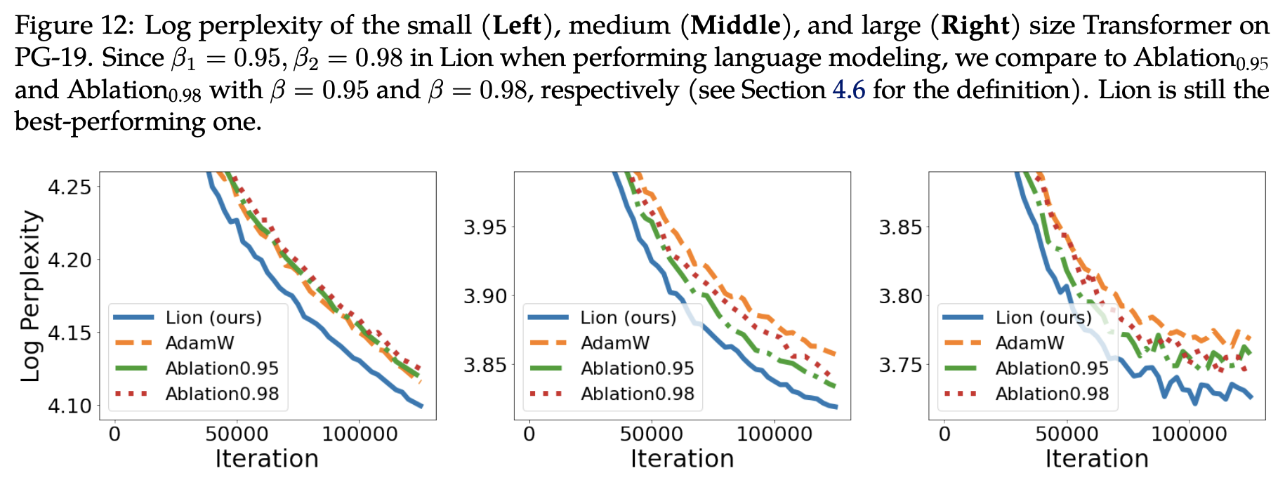Comparison of Lion, Tiger (Ablation), and AdamW on language modeling tasks

Here, Ablation0.95 and Ablation0.98 correspond to Tiger with $\beta$ set to 0.95 and 0.98, respectively. As you can see, on the small-size model, both Tiger variants are on par with AdamW, while on the middle and large-size models, both Tiger variants surpass AdamW. But as noted earlier, taking $\beta$ as the average of the two, 0.965, might yield further improvement.

As for CV tasks, the original paper gives Table 7:

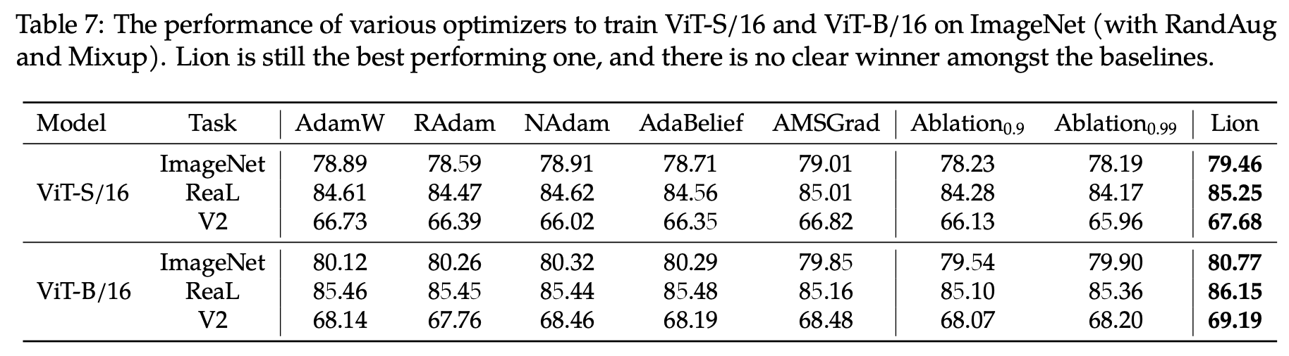Comparison of Lion, Tiger (Ablation), and AdamW on image classification tasks

Likewise, here Ablation0.9 and Ablation0.99 correspond to Tiger with $\beta$ set to 0.9 and 0.99. In this table, there's a noticeable gap between Tiger and AdamW. But considering that the authors only tested two values of $\beta$ — 0.9 and 0.99 — while I recommend $\beta=0.945$, I got in touch with the original authors and asked them to run supplementary experiments. Their reply was that "with $\beta$ set to 0.92, 0.95, and 0.98, the ImageNet results on ViT-B/16 are all around 80.0%." Comparing this to the figure above, we can conclude that with a well-tuned $\beta$, Tiger should also be able to match AdamW on CV tasks.

Finally, my own experiments. I usually use the LAMB optimizer, whose performance is roughly on par with AdamW but which is relatively more stable and adapts better to different initializations, so I've been happier using LAMB. Notably, LAMB's learning-rate settings can be carried over to Tiger without any changes. I retrained my earlier base-size GAU-α model using Tiger, and the training curves compared to before look like this:

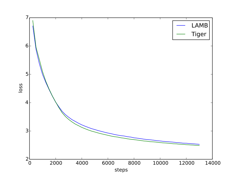My comparative experiment on GAU-α (loss curve)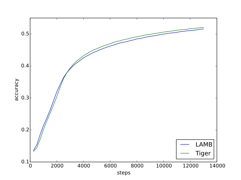My comparative experiment on GAU-α (accuracy curve)

As you can see, Tiger indeed achieves better performance than LAMB.

Future Work

Is there room to improve Tiger further? Certainly. There are actually quite a few ideas, but I haven't had time to validate them all — anyone interested is welcome to keep pushing on them.

In Google's Newly Discovered Optimizer Lion: A "Training Lion" with Both Efficiency and Effectiveness, I evaluated the $\text{sign}$ operation as follows:

By using the $\text{sign}$ operation, Lion treats every component equally, allowing the model to make full use of every component and thereby achieve better generalization. In SGD, the size of an update is proportional to its gradient; but some components have small gradients simply because they weren't initialized well, not because they're unimportant. So Lion's $\text{sign}$ operation gives every parameter a chance to "recover its vigor" or even "shine again."

On closer reflection, though, there's room for improvement here. "Treating every component equally" makes a lot of sense at the beginning of training, since it preserves as many possibilities for the model as possible. But if a particular parameter's gradient stays small for a long time, it's quite possible that this parameter really is a "lost cause" — i.e., it has already been optimized to its limit. If we still "treat every component equally" at that point, it becomes unfair to the "high achiever" components whose gradients remain large, and it can easily lead to oscillation in the model.

An intuitively appealing idea is that the optimizer should gradually degenerate from Tiger into SGD as training progresses. To this end, we could consider setting the update to

\begin{equation}\boldsymbol{u}_t = \text{sign}(\boldsymbol{m}_t) \times |\boldsymbol{m}_t|^{1-\gamma_t}\end{equation}

Here, both the absolute value and the power operation are element-wise, and $\gamma_t$ is a function monotonically decreasing from 1 to 0. When $\gamma_t=1$, this reduces to Tiger; when $\gamma_t = 0$, it reduces to SGDM.

Readers might complain that this introduces yet another schedule, $\gamma_t$, that needs tuning, making things more complicated. That's true — if we tune it independently, it would indeed introduce too much extra complexity. But let's think again: setting aside the warmup phase, isn't the relative learning rate $\alpha_t$, in general, itself a function monotonically decreasing to zero? Could we design $\gamma_t$ by borrowing from $\alpha_t$? For instance, isn't $\alpha_t/\alpha_0$ exactly a function monotonically decreasing from 1 to 0? Could we use it directly as $\gamma_t$? Of course, it's also possible that $(\alpha_t/\alpha_0)^2$ or $\sqrt{\alpha_t/\alpha_0}$ would work better — there's still room to tune — but at least we wouldn't need to design a whole new schedule spanning the entire training process from scratch.

Taking this further: since we sometimes use non-monotonic learning-rate schedules too (e.g., cosine annealing with restarts), could $\gamma_t$ also be non-monotonic (effectively switching back and forth between Tiger and SGDM)? These are all ideas that remain to be validated.

Summary

In this post, we introduced a new optimizer called Tiger (Tight-fisted Optimizer), which simplifies Lion and incorporates some of our hyperparameter-tuning experience. In particular, in scenarios that require gradient accumulation, Tiger achieves the theoretically optimal (and most "stingy") solution in terms of memory footprint!