GAN Models from an Energy Perspective (III): Generative Models = Energy Models
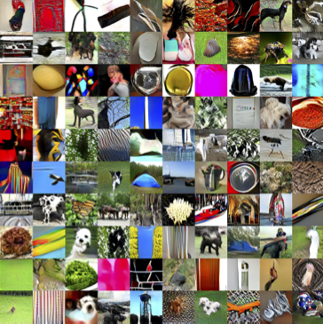 Conditional generation results of this paper's model on ImageNet (128x128)
The result I want to introduce today is still related to energy-based models; it comes from the paper Implicit Generation and Generalization in Energy-Based Models. Admittedly, this one no longer has much to do with GANs, but it's closely related to the energy-based model discussed in the second post of this series, so I'll still file it under this series.
I originally noticed this paper because of a report by Jiqizhixin, MIT Undergraduate Genius Reboots Energy-Based Generative Models, New Framework Rivals GANs. But honestly, this paper isn't all that interesting — to put it bluntly, it's a bit of a rehash, and the media headline actually got it right: it's a "reboot." The paper basically points out that an energy-based model is really just the stationary solution of a particular Langevin equation, and then uses this Langevin equation to perform sampling; once you have a sampling procedure, you can train the energy-based model. All of this theory is already well established, so I myself had thought along these lines back when I was studying stochastic differential equations, and I'm sure many others have too. So I think the authors' real contribution is that they took this rather straightforward idea and, through a series of training tricks, actually made it work.
Still, whatever the case, getting it to actually train is no small feat. And for readers who haven't looked into this topic before, it does serve as a solid case study of an energy-based model. So let me organize the overall approach of the paper so that readers can get a fuller picture of energy-based models. more
Energy Distributions
As in GAN Models from an Energy Perspective (II): GAN = "Analysis" + "Sampling", suppose we have a batch of data $x_1,x_2,\dots,x_n\sim p(x)$, which we want to fit using a probabilistic model. The model we choose is
\begin{equation}q_{\theta}(x) = \frac{e^{-U_{\theta}(x)}}{Z_{\theta}}\end{equation}
where $U_{\theta}$ is an undetermined function with parameters $\theta$, which we call the "energy function," and $Z_{\theta}$ is the normalizing factor (partition function)
\begin{equation}Z_{\theta} = \int e^{-U_{\theta}(x)}dx\label{eq:z}\end{equation}
Such a distribution can be called an "energy distribution," and in physics it is also known as the Boltzmann distribution.
To determine the parameters $\theta$, we first define the log-likelihood function:
\begin{equation}\mathbb{E}_{x\sim p(x)} \big[\log q_{\theta}(x)\big]\end{equation}
We want this to be as large as possible, i.e., we want
\begin{equation}L_{\theta}=\mathbb{E}_{x\sim p(x)} \big[-\log q_{\theta}(x)\big]\end{equation}
to be as small as possible. To this end, we apply gradient descent with respect to $L_{\theta}$. We have (see the second post for the detailed derivation)
\begin{equation}\nabla_{\theta}\log q_{\theta}(x)=-\nabla_{\theta} U_{\theta}(x)+\mathbb{E}_{x\sim q_{\theta}(x)}\big[\nabla_{\theta} U_{\theta}(x)\big]\end{equation}
so
\begin{equation}\nabla_{\theta} L_{\theta} = \mathbb{E}_{x\sim p(x)}\big[\nabla_{\theta} U_{\theta}(x)\big] - \mathbb{E}_{x\sim q_{\theta}(x)}\big[\nabla_{\theta} U_{\theta}(x)\big]\label{eq:q-grad}\end{equation}
which means the gradient descent update rule is
\begin{equation}\theta \leftarrow \theta - \varepsilon \Big(\mathbb{E}_{x\sim p(x)}\big[\nabla_{\theta} U_{\theta}(x)\big] - \mathbb{E}_{x\sim q_{\theta}(x)}\big[\nabla_{\theta} U_{\theta}(x)\big]\Big)\end{equation}
The Langevin Equation
In equation $\eqref{eq:q-grad}$, $\mathbb{E}_{x\sim p(x)}\big[\nabla_{\theta} U_{\theta}(x)\big]$ is easy to estimate — just sample a batch of real data and compute it directly. But $\mathbb{E}_{x\sim q_{\theta}(x)}\big[\nabla_{\theta} U_{\theta}(x)\big]$ is difficult, because we don't know how to sample from $q_{\theta}(x)$.
The approach in GAN Models from an Energy Perspective (II): GAN = "Analysis" + "Sampling" was to define another, easily sampled distribution $q_{\varphi}(x)$, and instead sample from $q_{\varphi}(x)$ while simultaneously shrinking the gap between $q_{\varphi}(x)$ and $q_{\theta}(x)$, so that $q_{\varphi}(x)$ can genuinely serve as a good approximation of $q_{\theta}(x)$. But this paper does something different: it samples directly from the Langevin equation corresponding to the energy-based model.
Actually the idea is quite simple, and I already mentioned it in the previous post. For the Langevin equation:
\begin{equation}x_{t+1} = x_t - \frac{1}{2}\varepsilon \nabla_x U(x_t) + \sqrt{\varepsilon}\alpha,\quad \alpha \sim \mathcal{N}(\alpha;0,1)\label{eq:sde}\end{equation}
when $\varepsilon\to 0$ and $t\to\infty$, the distribution followed by the sequence $\{x_t\}$ is exactly $q_{\theta}(x)$. In other words, $q_{\theta}(x)$ is the stationary distribution of this Langevin equation — or to put it yet another way, once $U_{\theta}(x)$ is given (which also fixes $q_{\theta}(x)$), the recursive process of equation $\eqref{eq:sde}$ can produce for us a batch of samples drawn from $q_{\theta}(x)$.
Well, once we have this sampling procedure, we're basically done: first, $\mathbb{E}_{x\sim q_{\theta}(x)}\big[\nabla_{\theta} U_{\theta}(x)\big]$ can now be estimated, so the energy-based model can be trained; and once training is complete, equation $\eqref{eq:sde}$ once again helps us sample a batch of new samples from the model, completing the generation process.
Model Details
Of course, that's the theory — in practice there are inevitably many details to work out, and no shortage of tricks required. When I originally thought this through, I stopped at this point, feeling that there were too many messy edge cases to resolve. But the authors pushed through and eventually got it working, which I genuinely admire.
First, the authors added spectral normalization to the model $U_{\theta}(x)$. Since $U_{\theta}(x)$ itself plays a role analogous to the discriminator in a GAN, adding spectral normalization makes sense. Second, during training, the energy function actually used is not $U_{\theta}(x)$ itself, but that plus a small L2 regularization term: $U_{\theta}(x) + \lambda U_{\theta}^2(x)$, where $\lambda$ is a small positive constant. According to the authors, this makes the overall loss smoother and training more stable (at inference time, $U_{\theta}(x)$ is still used).
Next, returning to the sampling issue: sampling is carried out via equation $\eqref{eq:sde}$, which is an iterative process, and an iterative process needs an initial value. However, if the initial value is drawn directly from some random distribution (such as a uniform distribution), the authors note that a mode-collapse-like problem arises — the images produced through the iteration end up looking too similar, leading to insufficiently diverse sampling. So the authors maintain a Buffer that caches historical sampling results, to be used as candidate initial values for the next round of sampling.
Overall, the model's update procedure is as follows:
Let the data sample distribution be $p(x)$. Choose a step size $\varepsilon$ (reference value 1/200), a number of iteration steps $K$ (reference value 20-50), and batch size $N$. Let the Buffer be denoted $\mathcal{B}$, initialized as an empty set.
Repeat until convergence:
Repeat to obtain a batch of real and fake samples:
1. Sample a real sample $x_r$ from $p(x)$ and add it to the current batch;
2. With 95% probability, select a sample from $\mathcal{B}$ as the initial value $x_{f,0}$ (or with 5% probability, draw it from a uniform distribution);
3. Starting from initial value $x_{f,0}$, iterate equation $\eqref{eq:sde}$ for $K$ steps to obtain $x_{f,K}$;
4. Treat $x_{f,K}$ as the fake sample $x_f$, add it to the current batch, and also add it to $\mathcal{B}$.
Once we have the real and fake samples, perform one optimizer step, with objective:
$\frac{1}{N}\sum\limits_{x_r, x_f} \Big\{U_{\theta}(x_r) - U_{\theta}(x_f) + \lambda \big[U_{\theta}^2(x_r) - U_{\theta}^2(x_f)\big]\Big\}$
For sampling after training is complete, the Buffer must also be maintained, and to ensure diversity, the authors train the model several times independently, obtaining several models with different weights, and then sample from all of these models simultaneously, sharing and jointly maintaining a single Buffer. For other details, readers can just refer to the original paper directly — since I don't plan to reproduce it myself, I won't dig any deeper.
Author's implementation: https://github.com/openai/ebm_code_release
Personal Summary
Overall, I'd say this is a solid, workmanlike paper — decent but not outstanding. On one hand, the underlying idea and theory are well-established; the relationship between energy-based models and the Langevin equation was already known, so there's not much novelty there. On the other hand, actually overcoming the various implementation difficulties and genuinely making this idea work in practice is no easy task, and it reflects the authors' deep (alchemical) skill in the field of generative models. From the perspective of energy-based models, this can also be seen as offering a viable recipe for training complex energy-based models.
As for the results, one could say they rival GANs, or one could say they still fall short. The authors mainly ran experiments on Cifar10 and ImageNet, which are of course both quite challenging datasets — ordinary GANs often struggle to generate good results on them. Judging from the sample images, this method can indeed compete with most GANs, and on Cifar10 it clearly beats Glow outright. As for why I say it falls short: I feel the method is a bit too heavy on tricks and not elegant enough. For instance, the sampling approach driven by the Langevin equation feels somewhat shaky to me, and while the Buffer-maintaining trick works reasonably well in practice, it clearly has a strong flavor of engineering hackery...
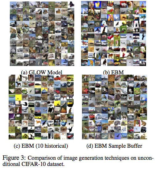 Results of unconditional generation on Cifar10
Translated automatically with claude-sonnet-5; all equations are reproduced verbatim from the source. Copyright remains with the original author.