From Denoising Autoencoders to Generative Models

从去噪自编码器到生成模型 苏剑林 · 2019-10-31 · Machine Learning generative model encoding gradient denoising

In my view, among the major conferences, ICLR papers are usually the most interesting, because their topics and style tend to be relaxed, playful, and full of unconventional ideas—the kind that really open your mind. So after the ICLR 2020 submission list came out, I took some time to skim through the papers, and indeed found quite a few interesting pieces of work.

Among them, I found two papers that use the idea of denoising autoencoders to build generative models: 《Learning Generative Models using Denoising Density Estimators》 and 《Annealed Denoising Score Matching: Learning Energy-Based Models in High-Dimensional Spaces》. Since I'm already fairly familiar with the conventional approaches to generative models, this "unconventional" line of thinking caught my attention. Reading closely, I found that the two papers share the same starting point, but differ in their concrete approach, and yet end up arriving at essentially the same conclusion—a rather beautiful case of "one problem, multiple solutions." So I've decided to put the two papers together and give a comparative analysis.

Denoising Autoencoding

Both papers fundamentally start from the denoising autoencoder—more precisely, they exploit the optimal solution of the denoising autoencoder.

Basic result: If $x,\varepsilon\in \mathbb{R}^d$, and $x\sim p(x),\varepsilon\sim u(\varepsilon)$, where $u(\varepsilon)=\mathcal{N}(0,\sigma^2 I_d)$, then
\begin{equation}\begin{aligned}r(x)=&\,\mathop{\text{argmin}}_{r}\mathbb{E}_{x\sim p(x),\varepsilon\sim \mathcal{N}(0,\sigma^2 I_d)}\left[\Vert r(x + \varepsilon) - x\Vert^2\right] \\ > =&\,x + \sigma^2 \nabla_x \,\log\hat{p}(x)\end{aligned}\label{eq:denoise}\end{equation}

Here $\hat{p}(x)=[p*u](x)=\int p(x-\varepsilon)u(\varepsilon) d\varepsilon=\int p(\varepsilon)u(x-\varepsilon) d\varepsilon$ denotes the convolution of distributions $p(x)$ and $u(\varepsilon)$; concretely, it is the probability density of $x+\varepsilon$. In other words, if $p(x)$ represents the distribution of real images, then if we could sample from $\hat{p}(x)$, we would obtain a batch of real images with Gaussian noise added.

Result $\eqref{eq:denoise}$ tells us that the optimal denoising autoencoder for additive Gaussian noise can be computed explicitly, and the result is related to the gradient of the distribution. This result is quite interesting, and rather profound—well worth savoring. For instance, equation $\eqref{eq:denoise}$ tells us that $r(x)-x$ is in fact an estimator of the gradient of the (noisy) true distribution, and once we have the gradient of the true distribution, we can actually do a lot of things, especially things related to generative models.

Proof:
The proof of $\eqref{eq:denoise}$ is actually not difficult. From the variational objective we get
\begin{equation}\begin{aligned}&\delta \iint p(x)u(\varepsilon)\left\Vert r(x + \varepsilon) - x\right\Vert_2^2 dx d\varepsilon\\ > =&\delta \iint p(x)u(y-x)\left\Vert r(y) - x\right\Vert_2^2 dx dy\\ > =&2\iint p(x)u(y-x)\left\langle r(y) - x, \delta r(y)\right\rangle dx dy\\ > \end{aligned}\end{equation}
so $\int p(x)u(y-x)(r(y) - x)dx=0$, i.e.
\begin{equation}r(y) = \frac{\int p(x)u(y-x)x dx}{\int p(x)u(y-x) dx}\end{equation}
Substituting into the expression $u(\varepsilon)=\frac{1}{(2\pi \sigma^2)^{d/2}}\exp\left(-\frac{\left\Vert\varepsilon\right\Vert_2^2}{2\sigma^2}\right)$, we obtain
\begin{equation}r(y) = y + \sigma^2\nabla_y \log\left[p*u\right](y)\end{equation}

A Winding Path to a Hidden Spot

Let's first introduce the approach of 《Learning Generative Models using Denoising Density Estimators》. Following the usual convention of GANs and VAEs, we want to train a mapping $x=G(z)$ such that samples $z$ drawn from the prior distribution $q(z)$ are all mapped to something resembling a real sample. In terms of probability, this means we want to bring $p(x)$ close to the following $q(x)$:

\begin{equation}q(x) = \int q(z)\delta(x - G_{\theta}(z))dz\end{equation}

To this end, the objective commonly used by GANs is to minimize $KL(q(x)\Vert p(x))$—this perspective can be found in 《Understanding Generative Models via Variational Inference: VAE, GAN, AAE, ALI》 and 《GANs from an Energy Perspective (II): GAN = "Analysis" + "Sampling"》. However, since what we estimated above is the gradient of $\hat{p}(x)$, we can instead adopt a different objective: minimize $KL\left(\hat{q}(x)\big\Vert \hat{p}(x)\right)$.

To do this, we can carry out the following derivation:

\begin{equation}\begin{aligned}KL\left(\hat{q}(x)\big\Vert \hat{p}(x)\right)=&\int \hat{q}(x) \log \frac{\hat{q}(x)}{\hat{p}(x)}dx\\ =&\int q(x)u(\varepsilon) \log \frac{\hat{q}(x+\varepsilon)}{\hat{p}(x+\varepsilon)}dx d\varepsilon\\ =&\int q(z)\delta(x-G_{\theta}(z))u(\varepsilon) \log \frac{\hat{q}(x+\varepsilon)}{\hat{p}(x+\varepsilon)}dx d\varepsilon dz\\ =&\int q(z)u(\varepsilon) \log \frac{\hat{q}(G_{\theta}(z)+\varepsilon)}{\hat{p}(G_{\theta}(z)+\varepsilon)}d\varepsilon dz\\ =&\,\mathbb{E}_{z\sim q(z), \varepsilon\sim u(\varepsilon)}\big[\log \hat{q}(G_{\theta}(z)+\varepsilon) - \log \hat{p}(G_{\theta}(z)+\varepsilon)\big]\\ \end{aligned}\label{eq:dae-1}\end{equation}

This objective requires us to obtain estimates of $\log\hat{p}(x)$ and $\log\hat{q}(x)$. We can build two $\mathbb{R}^d \to \mathbb{R}$ models, $E_p(x)$ and $E_q(x)$, using neural networks, and then minimize respectively

\begin{equation}\begin{aligned}\mathop{\text{argmin}}_{E_p}\mathbb{E}_{x\sim p(x),\varepsilon\sim \mathcal{N}(0,\sigma^2 I_d)}\left[\Vert \nabla_x E_p(x + \varepsilon) + \varepsilon\Vert^2\right]\\ \mathop{\text{argmin}}_{E_q}\mathbb{E}_{x\sim q(x),\varepsilon\sim \mathcal{N}(0,\sigma^2 I_d)}\left[\Vert \nabla_x E_q(x + \varepsilon) + \varepsilon\Vert^2\right] \end{aligned}\label{eq:e-grad}\end{equation}

That is, we use $\nabla_x E_p(x)+x$ and $\nabla_x E_q(x)+x$ as denoising autoencoders. According to result $\eqref{eq:denoise}$, we then have

\begin{equation}\left\{\begin{aligned}\nabla_x E_p(x)+x=x+\sigma^2 \nabla_x \log \hat{p}(x)\\ \nabla_x E_q(x)+x=x+\sigma^2 \nabla_x \log \hat{q}(x)\end{aligned}\right. \quad\Rightarrow\quad \left\{\begin{aligned}E_p(x) = \sigma^2 \log \hat{p}(x) + C_1\\ E_q(x) = \sigma^2 \log \hat{q}(x) + C_2\end{aligned}\right.\end{equation}

In other words, up to an additive constant, $E_p(x)$ is proportional to $\log \hat{p}(x)$, and $E_q(x)$ is proportional to $\log \hat{q}(x)$; and since the constant doesn't affect the optimization, we can substitute $E_p(x)$ and $E_q(x)$ into $\eqref{eq:dae-1}$, obtaining

\begin{equation}KL\left(\hat{q}(x)\big\Vert \hat{p}(x)\right)\sim\,\mathbb{E}_{z\sim q(z), \varepsilon\sim u(\varepsilon)}\big[E_q(G_{\theta}(z)+\varepsilon) - E_p(G_{\theta}(z)+\varepsilon)\big]\label{eq:dae-2}\end{equation}

This gives us the following procedure for a generative model:

Choose a prior distribution $q(z)$, initialize $G_{\theta}(z)$, and precompute $E_p(x)$. Repeat the following 3 steps until convergence:
1. Sample a batch of $z\sim q(z)$, sample a batch of noise $\varepsilon\sim\mathcal{N}(0,\sigma^2 I_d)$, and combine them to form a batch of noisy fake samples $x = G_{\theta}(z)+\varepsilon$;
2. Use this batch of noisy fake samples to train $E_q(x)$;
3. Fix $E_p,E_q$, and use gradient descent based on $\eqref{eq:dae-2}$ to update $G_{\theta}$ for several steps;

The experiments in this paper are fairly simple, only covering MNIST and Fashion-MNIST, demonstrating the feasibility of the approach:

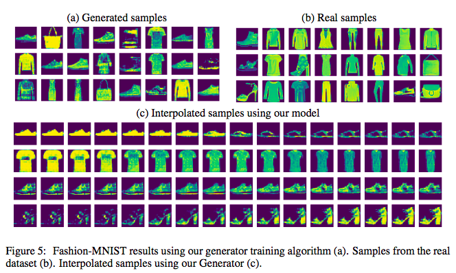Generation results on Fashion-MNIST

A Twist in the Road

The other paper, 《Annealed Denoising Score Matching: Learning Energy-Based Models in High-Dimensional Spaces》, is even more blunt and direct—it's essentially a combination of the denoising autoencoder idea with 《GANs from an Energy Perspective (III): Generative Model = Energy Model》.

Since $\eqref{eq:denoise}$ has already given us $\nabla_x\log\hat{p}(x)=(r(x)-x)/\sigma^2$ (although in practice this paper doesn't directly fit $r(x)$ with a neural network, but rather, like $\eqref{eq:e-grad}$, fits a scalar function with a neural network—this doesn't change the underlying idea), this actually already lets us sample from $\hat{p}(x)$. Of course, the resulting images will be noisy, so we still need to feed the sampled results through $r(x)$ to denoise them, i.e.

$$p(x) = \mathbb{E}_{x_{noise}\sim \hat{p}(x)} \big[\delta(x - r(x_{noise}))\big]$$

So concretely, how do we sample from $\hat{p}(x)$? The Langevin equation! Since we already know $\nabla_x\log\hat{p}(x)$, the following Langevin equation

\begin{equation}x_{t+1} = x_t + \frac{1}{2}\varepsilon \nabla_x\log\hat{p}(x) + \sqrt{\varepsilon}\alpha,\quad \alpha \sim \mathcal{N}(\alpha;0,1)\label{eq:sde}\end{equation}

when $\varepsilon\to 0$ and $t\to\infty$, has a sequence $\{x_t\}$ that follows the distribution obtained by sampling from $\hat{p}(x)$. In other words, $\hat{p}(x)$ is the stationary distribution of this Langevin equation.

So the process of sampling from $\hat{p}(x)$ is resolved by 《Annealed Denoising Score Matching: Learning Energy-Based Models in High-Dimensional Spaces》 using this rather blunt and direct (though, in my opinion, not particularly elegant) method. As a result, once the denoising autoencoder is trained, one automatically obtains a generative model...

The overall procedure is:

1. Train a denoising autoencoder $r(x)$, obtaining $\nabla_x\hat{p}(x)$;
2. Use the iterative process $\eqref{eq:sde}$ to sample, yielding a batch of noisy real samples;
3. Pass the samples obtained in step 2 through $r(x)$ to denoise them, obtaining noise-free samples.

Of course, the paper contains many more details—its core technique is the use of an annealing trick to stabilize training and improve generation quality—but I'm not particularly interested in those details, since my main goal here is just to learn some novel ideas about generative models and broaden my horizons. That said, I have to admit that even though the method feels somewhat crude, the generation quality of this paper is still fairly competitive, achieving quite good results on Fashion-MNIST, CelebA, and CIFAR-10:

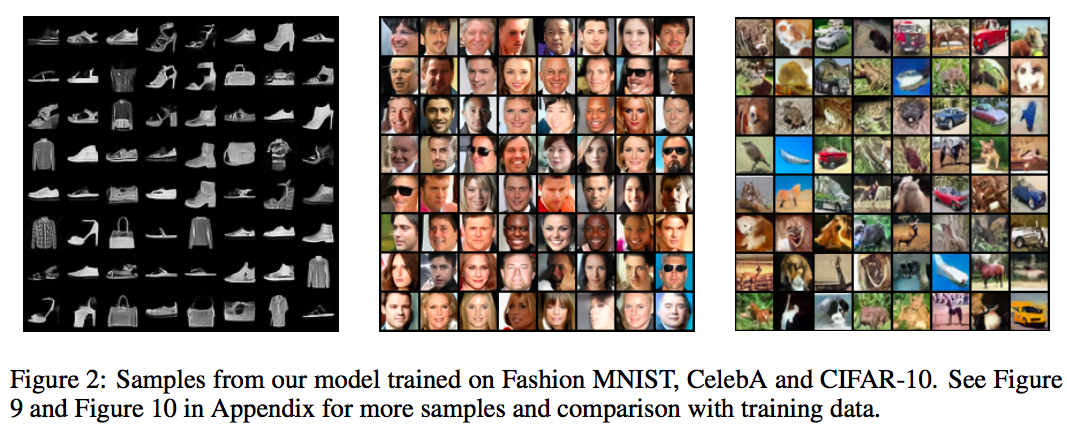Generation results on Fashion-MNIST, CelebA, and CIFAR-10

As the Curtain Falls

This post introduced two similar papers submitted to ICLR 2020, both of which use denoising autoencoders to build generative models. Since I hadn't come across this line of thinking before, I read through them side by side with considerable interest.

Setting aside the actual generation quality, I think both are quite thought-provoking, and they've sparked some reflections for me (not just in CV, but also in NLP). For instance, BERT's MLM pretraining scheme is essentially also a denoising autoencoder—so is there some analogous result to $\eqref{eq:denoise}$? Or conversely, could a result like $\eqref{eq:denoise}$ inspire us to design new pretraining tasks, or perhaps even help us clarify the underlying principle behind the pretrain + finetune paradigm?