A Steady Stream of Flow: TARFLOW - Flow Models Return in Full Force?

细水长flow之TARFLOW：流模型满血归来？ 苏剑林 · 2025-01-17 · Machine Learning flow model flow generative model attention

I wonder if any readers still remember this series? It's called "A Long Trickle of Flow" (细水长flow), and it's mainly about flow-based models. It started back in 2018, when OpenAI released a new flow model, Glow, which was genuinely dazzling at a time when GANs dominated the field. But dazzling as it was, for quite a long time Glow and its subsequent improvements never matched GANs in terms of generation quality — let alone today's mainstream diffusion models.

That situation may be about to change, though. Last month's paper Normalizing Flows are Capable Generative Models proposes a new flow model called TARFLOW, which comes close to current SOTA on almost every generation task — a full-strength comeback for flow models, if you will.

Before We Begin

The "flow models" discussed here specifically refer to Normalizing Flows: work characterized by an invertible model architecture, trained with maximum likelihood, capable of one-step generation. Flow Matching, a branch of current diffusion models, is not included in this category.

Ever since Glow's dazzling debut, subsequent progress on flow models has been, frankly, "unremarkable." To put it simply, it was hard even to generate CelebA faces without obvious artifacts, let alone tackle something as complex as ImageNet. That's why the "A Long Trickle of Flow" series stopped back in 2019 with A Long Trickle of Flow: Invertible ResNets and the Aesthetics of Extreme Brute Force. But the arrival of TARFLOW proves that flow models "still have some fight left in them." Here's what its generated images look like this time around:

TARFLOW generation results

By comparison, here's what Glow's generated images used to look like:

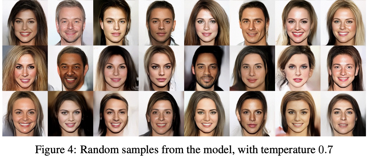Glow generation results

Glow was only demonstrating relatively simple face generation, yet the artifacts are already quite obvious — let alone the more complex task of natural image generation. This shows that TARFLOW's progress is no small matter. Quantitatively speaking, its performance also approaches the best models around, surpassing BigGAN, the SOTA representative of GANs:

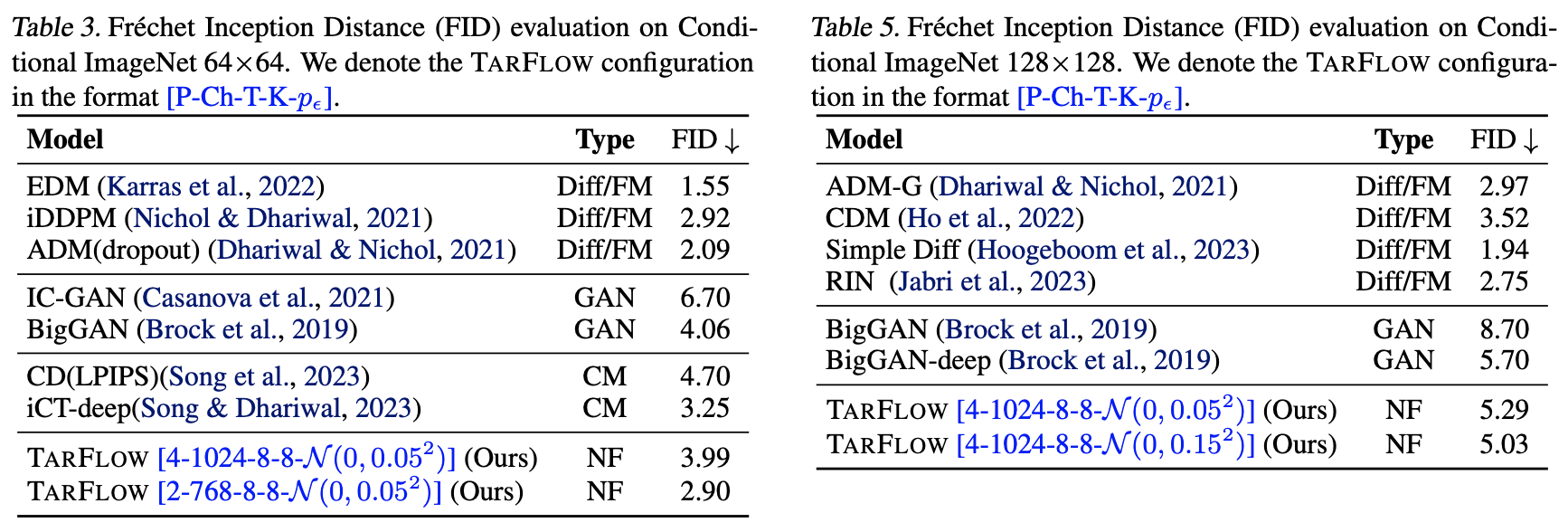Quantitative comparison of TARFLOW against other models

Keep in mind, flow models are inherently one-step generative models, and unlike GANs they don't require adversarial training — they're trained end-to-end with a single loss function, which in some sense makes their training even simpler than diffusion models. So the fact that TARFLOW has raised the bar for flow model quality means it now combines the advantages of both GANs and diffusion models, while retaining its own unique strengths (invertibility, the ability to estimate log-likelihood, and so on).

Model Recap

Getting back on track, let's look at what "miracle cure" TARFLOW used to revitalize flow models. But before that, let's briefly review the theoretical foundations of flow models; for a more detailed historical account, see A Long Trickle of Flow: NICE — Basic Concepts and Implementation of Flow Models and A Long Trickle of Flow: RealNVP and Glow — Inheritance and Refinement of Flow Models.

Ultimately, both flow models and GANs aim to obtain a deterministic function $\boldsymbol{x}=\boldsymbol{g}_{\boldsymbol{\theta}}(\boldsymbol{z})$ that maps random noise $\boldsymbol{z}\sim\mathcal{N}(\boldsymbol{0},\boldsymbol{I})$ to images $\boldsymbol{x}$ from the target distribution. In the language of probability distributions, this means modeling the target distribution with a distribution of the following form:

\begin{equation}q_{\boldsymbol{\theta}}(\boldsymbol{x}) = \int \delta(\boldsymbol{x} - \boldsymbol{g}_{\boldsymbol{\theta}}(\boldsymbol{z}))q(\boldsymbol{z})d\boldsymbol{z}\label{eq:q-int}\end{equation}

where $q(\boldsymbol{z}) = \mathcal{N}(\boldsymbol{0},\boldsymbol{I})$, and $\delta()$ is the Dirac delta function. The ideal training objective for a probabilistic model is maximum likelihood, i.e., using $-\log q_{\boldsymbol{\theta}}(\boldsymbol{x})$ as the loss function. But the current form of $q_{\boldsymbol{\theta}}(\boldsymbol{x})$ contains an integral and only has formal meaning — it can't actually be used for training.

This is where flow models and GANs "part ways": GANs, roughly speaking, use another model (a discriminator) to approximate $-\log q_{\boldsymbol{\theta}}(\boldsymbol{x})$, which leads to alternating training. Flow models instead design an appropriate $\boldsymbol{g}_{\boldsymbol{\theta}}(\boldsymbol{z})$ so that the integral $\eqref{eq:q-int}$ can be computed directly. What conditions are needed to compute the integral $\eqref{eq:q-int}$ directly? Let $\boldsymbol{y} = \boldsymbol{g}_{\boldsymbol{\theta}}(\boldsymbol{z})$, with inverse function $\boldsymbol{z} = \boldsymbol{f}_{\boldsymbol{\theta}}(\boldsymbol{y})$. Then

\begin{equation}d\boldsymbol{z} = \left|\det \frac{\partial \boldsymbol{z}}{\partial \boldsymbol{y}}\right|d\boldsymbol{y} = \left|\det \frac{\partial \boldsymbol{f}_{\boldsymbol{\theta}}(\boldsymbol{y})}{\partial \boldsymbol{y}}\right|d\boldsymbol{y}\end{equation}

and

\begin{equation}\begin{aligned} q_{\boldsymbol{\theta}}(\boldsymbol{x}) =&\, \int \delta(\boldsymbol{x} - \boldsymbol{g}_{\boldsymbol{\theta}}(\boldsymbol{z}))q(\boldsymbol{z})d\boldsymbol{z} \\ =&\, \int \delta(\boldsymbol{x} - \boldsymbol{y})q(\boldsymbol{f}_{\boldsymbol{\theta}}(\boldsymbol{y}))\left|\det \frac{\partial \boldsymbol{f}_{\boldsymbol{\theta}}(\boldsymbol{y})}{\partial \boldsymbol{y}}\right|d\boldsymbol{y} \\ =&\, q(\boldsymbol{f}_{\boldsymbol{\theta}}(\boldsymbol{x}))\left|\det \frac{\partial \boldsymbol{f}_{\boldsymbol{\theta}}(\boldsymbol{x})}{\partial \boldsymbol{x}}\right| \end{aligned}\end{equation}

therefore

\begin{equation}-\log q_{\boldsymbol{\theta}}(\boldsymbol{x}) = -\log q(\boldsymbol{f}_{\boldsymbol{\theta}}(\boldsymbol{x})) - \log \left|\det \frac{\partial \boldsymbol{f}_{\boldsymbol{\theta}}(\boldsymbol{x})}{\partial \boldsymbol{x}}\right|\end{equation}

This shows that computing the integral $\eqref{eq:q-int}$ requires two things: first, knowing the inverse function $\boldsymbol{z} = \boldsymbol{f}_{\boldsymbol{\theta}}(\boldsymbol{x})$ of $\boldsymbol{x} = \boldsymbol{g}_{\boldsymbol{\theta}}(\boldsymbol{z})$; second, being able to compute the determinant of the Jacobian matrix $\frac{\partial \boldsymbol{f}_{\boldsymbol{\theta}}(\boldsymbol{x})}{\partial \boldsymbol{x}}$.

Affine Coupling

To this end, flow models introduce a key design — the "affine coupling layer":

\begin{equation}\begin{aligned}&\boldsymbol{h}_1 = \boldsymbol{x}_1\\ &\boldsymbol{h}_2 = \exp(\boldsymbol{\gamma}(\boldsymbol{x}_1))\otimes\boldsymbol{x}_2 + \boldsymbol{\beta}(\boldsymbol{x}_1)\end{aligned}\label{eq:couple}\end{equation}

where $\boldsymbol{x} = [\boldsymbol{x}_1,\boldsymbol{x}_2]$, and $\boldsymbol{\gamma}(\boldsymbol{x}_1)$, $\boldsymbol{\beta}(\boldsymbol{x}_1)$ are models that take $\boldsymbol{x}_1$ as input and produce output with the same shape as $\boldsymbol{x}_2$, and $\otimes$ denotes the Hadamard product. What this equation says is: split $\boldsymbol{x}$ into two parts (the split can be arbitrary, not necessarily even), leave one part unchanged in the output, and transform the other part according to a specified rule. Note that the affine coupling layer is invertible, with inverse

\begin{equation}\begin{aligned}&\boldsymbol{x}_1 = \boldsymbol{h}_1\\ &\boldsymbol{x}_2 = \exp(-\boldsymbol{\gamma}(\boldsymbol{h}_1))\otimes(\boldsymbol{h}_2 - \boldsymbol{\beta}(\boldsymbol{h}_1))\end{aligned}\end{equation}

This satisfies the first condition, invertibility. On the other hand, the Jacobian matrix of the affine coupling layer is lower triangular:

\begin{equation}\frac{\partial \boldsymbol{h}}{\partial \boldsymbol{x}} = \begin{pmatrix}\frac{\partial \boldsymbol{h}_1}{\partial \boldsymbol{x}_1} & \frac{\partial \boldsymbol{h}_1}{\partial \boldsymbol{x}_2} \\ \frac{\partial \boldsymbol{h}_2}{\partial \boldsymbol{x}_1} & \frac{\partial \boldsymbol{h}_2}{\partial \boldsymbol{x}_2}\end{pmatrix}=\begin{pmatrix}\boldsymbol{I} & \boldsymbol{O} \\ \frac{\partial (\exp(\boldsymbol{\gamma}(\boldsymbol{x}_1))\otimes\boldsymbol{x}_2 + \boldsymbol{\beta}(\boldsymbol{x}_1))}{\partial \boldsymbol{x}_1} & \text{diag}(\exp(\boldsymbol{\gamma}(\boldsymbol{x}_1)))\end{pmatrix}\end{equation}

The determinant of a triangular matrix equals the product of its diagonal entries, so

\begin{equation}\log\left|\det\frac{\partial \boldsymbol{h}}{\partial \boldsymbol{x}}\right| = \sum_i \boldsymbol{\gamma}_i(\boldsymbol{x}_1)\end{equation}

That is, the log absolute value of the Jacobian determinant equals the sum of the components of $\boldsymbol{\gamma}(\boldsymbol{x}_1)$, which satisfies the second condition — computability of the Jacobian determinant.

The affine coupling layer was first proposed in RealNVP, where NVP stands for "Non-Volume Preserving." This name is contrasted with the special case where $\boldsymbol{\gamma}(\boldsymbol{x}_1)$ is identically zero, called an "additive coupling layer," which was proposed in NICE. Its distinguishing feature is that its Jacobian determinant equals 1, meaning the additive coupling layer is "volume-preserving" (the determinant's geometric meaning being volume).

Note that if we simply stack multiple affine coupling layers, $\boldsymbol{x}_1$ will remain unchanged throughout — which is not what we want. What we actually want to do is map the entirety of $\boldsymbol{x}$ to a standard normal distribution. To solve this problem, before applying each affine coupling layer, we need to "shuffle" the input components in some way, so as to avoid components that never change. The "shuffle" operation corresponds to a permutation matrix transformation, whose determinant's absolute value is always 1.

The Core Improvement

Everything up to this point has just been basic background on flow models — now let's get to TARFLOW's actual contribution.

First, TARFLOW notes that the affine coupling layer $\eqref{eq:couple}$ can be generalized to a multi-block partition, i.e., splitting $\boldsymbol{x}$ into more parts $[\boldsymbol{x}_1,\boldsymbol{x}_2,\cdots,\boldsymbol{x}_n]$, and applying a similar rule:

\begin{equation}\begin{aligned}&\boldsymbol{h}_1 = \boldsymbol{x}_1\\ &\boldsymbol{h}_k = \exp(\boldsymbol{\gamma}_k(\boldsymbol{x}_{< k}))\otimes\boldsymbol{x}_k + \boldsymbol{\beta}_k(\boldsymbol{x}_{< k})\end{aligned}\label{eq:couple-2}\end{equation}

where $k > 1$, $\boldsymbol{x}_{< k}=[\boldsymbol{x}_1,\boldsymbol{x}_2,\cdots,\boldsymbol{x}_{k-1}]$, with inverse operation

\begin{equation}\begin{aligned}&\boldsymbol{x}_1 = \boldsymbol{h}_1\\ &\boldsymbol{x}_k = \exp(-\boldsymbol{\gamma}_k(\boldsymbol{x}_{< k}))\otimes(\boldsymbol{h}_k - \boldsymbol{\beta}_k(\boldsymbol{x}_{< k}))\end{aligned}\label{eq:couple-2-inv}\end{equation}

Similarly, the log absolute value of the Jacobian determinant of this generalized affine coupling layer equals the sum of all components of $\boldsymbol{\gamma}_2(\boldsymbol{x}_{< 2}),\cdots,\boldsymbol{\gamma}_n(\boldsymbol{x}_{< n})$, so both conditions required by flow models are satisfied. The prototype of this generalization was actually proposed as early as 2016, in IAF, even earlier than Glow.

So why did so little subsequent work explore this direction further? This is largely for historical reasons. In earlier years, the dominant architecture for CV models was CNNs, and using a CNN presupposes that features exhibit local correlation. This meant that when partitioning $\boldsymbol{x}$ into blocks, people tended to only consider splitting along the channel dimension. This is because each layer also requires a necessary shuffling operation — once you choose to split along the two spatial dimensions (height and width), the random shuffle would destroy local correlation in the features, making CNNs unusable. And if you split into multiple parts along the channel dimension instead, then it becomes difficult for the multiple channel feature maps to interact efficiently.

However, in the era of Transformers, the situation is completely different. The input to a Transformer is essentially an unordered set of vectors — in other words, it doesn't rely on local correlation. So with a Transformer as the main architecture, we're free to split along the spatial dimensions, which is exactly what Patchify does. Moreover, the form $\boldsymbol{h}_{k} = \cdots(\boldsymbol{x}_{< k})$ in equation $\eqref{eq:couple-2}$ implies that this is a causal model, which also happens to be efficiently implementable with a Transformer.

Beyond this formal compatibility, what fundamental benefit does splitting along the spatial dimensions bring? This brings us back to the goal of flow models: $\boldsymbol{g}_{\boldsymbol{\theta}}(\boldsymbol{z})$ turns noise into images, while the inverse model $\boldsymbol{f}_{\boldsymbol{\theta}}(\boldsymbol{x})$ turns images into noise. The defining property of noise is randomness — plainly put, it's disorder — whereas the defining property of images is local correlation. So one key to turning images into noise is disrupting this local correlation, and directly Patchifying along the spatial dimensions, combined with the shuffling operation already built into the coupling layer, is undoubtedly the most efficient choice.

So equation $\eqref{eq:couple-2}$ and the Transformer are a natural match — "hitting it off at first sight," so to speak, and mutually reinforcing one another. This is what the "TAR" in TARFLOW stands for (Transformer AutoRegressive Flow), and it's also TARFLOW's core innovation.

Adding and Removing Noise

A common training trick for flow models is noise injection — that is, adding a small amount of noise to images before feeding them into the model for training. Although we treat images as continuous vectors, they're actually stored in discrete format, and noise injection helps smooth out this discontinuity, making images closer to true continuous vectors. Adding noise also prevents the model from over-relying on specific details in the training data, thereby reducing the risk of overfitting.

Noise injection is a standard operation for flow models and wasn't first proposed by TARFLOW. What TARFLOW does propose is denoising. In theory, a flow model trained on noise-injected images will also produce noisy generation results — it's just that previous flow models weren't performing well enough for this residual noise to matter much. But once TARFLOW pushed flow model performance up, denoising became "imperative," or else the noise would become the main factor limiting quality.

So how do we denoise? Should we train a separate denoising model? That's not actually necessary. We already proved in From Denoising Autoencoders to Generative Models that if $q_{\boldsymbol{\theta}}(\boldsymbol{x})$ is the probability density function trained after adding noise $\mathcal{N}(\boldsymbol{0},\sigma^2 \boldsymbol{I})$, then

\begin{equation}\boldsymbol{r}(\boldsymbol{x}) = \boldsymbol{x} + \sigma^2 \nabla_{\boldsymbol{x}} \log q_{\boldsymbol{\theta}}(\boldsymbol{x})\end{equation}

is the theoretically optimal solution for the denoising model. So once we have $q_{\boldsymbol{\theta}}(\boldsymbol{x})$, there's no need to train an additional denoising model — we can just compute the above expression directly to denoise. This is another advantage of flow models. And precisely because a denoising step is incorporated, TARFLOW switched its input noise to a Gaussian distribution and appropriately increased the noise variance, which is another reason for its improved performance.

Putting all this together, TARFLOW's complete sampling procedure is:

\begin{equation}\boldsymbol{z}\sim \mathcal{N}(\boldsymbol{0},\boldsymbol{I}) ,\quad \boldsymbol{y} =\boldsymbol{g}_{\boldsymbol{\theta}}(\boldsymbol{z}),\quad\boldsymbol{x} = \boldsymbol{y} + \sigma^2 \nabla_{\boldsymbol{y}} \log q_{\boldsymbol{\theta}}(\boldsymbol{y}) \end{equation}

Further Thoughts

That covers the key changes in TARFLOW compared to previous flow models. For the remaining model details, I'd encourage readers to consult the original paper — and if there's anything still unclear, the official open-source code is also available for reference.

GitHub: https://github.com/apple/ml-tarflow

Now let me share some of my own thoughts on TARFLOW.

First, it should be pointed out that although TARFLOW achieves SOTA results in terms of quality, its sampling speed actually falls short of expectations. The appendix of the original paper mentions that sampling 32 ImageNet64 images on an A100 takes about 2 minutes. Why is it so slow? If we take a close look at the inverse of the coupling layer $\eqref{eq:couple-2-inv}$, we'll notice that it's actually a nonlinear RNN! A nonlinear RNN can only be computed sequentially, and this is the fundamental reason for its slowness.

In other words, TARFLOW is essentially a model with fast training but slow sampling. Of course, if we wanted to, we could flip this around to get slow training but fast sampling instead — but either way, one direction, forward or inverse, is inevitably going to be slow. This is a drawback of the multi-block affine coupling layer, and it's also the main direction in which TARFLOW would want further improvement.

Second, the "AR" in TARFLOW might easily bring to mind today's mainstream autoregressive LLMs — so can the two be integrated to do multimodal generation? Honestly, this is difficult. TARFLOW's "AR" property is purely a requirement of the affine coupling layer, and since there's also a shuffling step before each coupling layer, it isn't actually a genuinely causal model — quite the opposite, it's thoroughly bidirectional. So it doesn't lend itself well to being forcibly integrated with the autoregressive nature of text generation.

Overall, if TARFLOW's sampling speed can be further improved, it would become a highly competitive pure vision generative model. Because beyond simple training and excellent performance, the invertibility of flow models offers yet another advantage: as described in The Reversible Residual Network: Backpropagation Without Storing Activations, backpropagation can be done without storing activations at all, and the cost of recomputation is much lower than for ordinary models.

As for whether it could become a unified architecture for multimodal LLMs — that's something we can't say clearly just yet.

A Renaissance

Finally, a few words on the "renaissance" of deep learning models.

In recent years, a fair amount of work has attempted to combine current understanding to revisit and improve models that seemed to have fallen out of favor, and has produced some interesting new results. Besides TARFLOW's attempt to revitalize flow models, there's also The GAN is dead; long live the GAN! A Modern GAN Baseline, which sifted through various combinations of GAN techniques to distill the essential ones and arrived at equally competitive results.

Even earlier, there's Improved Residual Networks for Image and Video Recognition and Revisiting ResNets: Improved Training and Scaling Strategies, which pushed ResNets to new heights, and even RepVGG: Making VGG-style ConvNets Great Again, which brought back the classic VGG. And of course, we shouldn't forget work on SSMs and linear attention, which represent something of a "renaissance" for RNNs.

Here's hoping this blossoming wave of "renaissance" gets even more vigorous — it will give us a fuller and more accurate understanding of these models.