The Endless Flow of NICE: Basic Concepts and Implementation of Flow Models

细水长flow之NICE：流模型的基本概念与实现 苏剑林 · 2018-08-11 · Machine Learning probability flow model flow generative model

Foreword: Ever since I read about the Glow model on Jiqizhixin (see "The Next GAN? OpenAI's Invertible Generative Model Glow"), I haven't been able to stop thinking about it. New machine learning models keep popping up all the time, and I usually keep an eye on such developments, but rarely does a model make my heart skip a beat the way Glow did — that feeling of "this is it." Even more surprisingly, this model, whose results looked so impressive, turned out to be something I'd never even heard of before. So I read through it over and over for several days, and the more I read, the more interesting I found it — it felt like it could tie together a lot of ideas I'd had before. Here, then, is a summary of where I've gotten to so far.

Background

This post is mainly an introduction to and implementation of NICE: Non-linear Independent Components Estimation. This paper is also one of the foundational works behind the Glow model — it's essentially the cornerstone on which Glow was built.

A Difficult Distribution

As is well known, the mainstream generative models today are VAEs and GANs, but in fact, beyond these two, there are also flow-based models (flow can be translated directly as "流"; we'll introduce the concept later). In fact, flow has a history just as long as VAEs and GANs, but it remains little known. In my view, the reason is probably that flow lacks an intuitive story like GAN's "counterfeiter vs. discriminator" — flow leans heavily mathematical, and early on its results weren't especially impressive while its computational cost was quite high, so it was hard for people to get excited about it. Now, however, it seems that OpenAI's astonishingly good, flow-based Glow model will likely draw more people into improving flow models.

High-resolution faces generated by the Glow model]

The essence of a generative model is that we want to fit the given data samples using a probability model we understand — that is, we need to write down a distribution $q_{\boldsymbol{\theta}}(\boldsymbol{x})$ with parameters $\boldsymbol{\theta}$. However, our neural networks are only "universal function approximators," not "universal distribution approximators." In principle, they can fit any function, but they cannot arbitrarily fit any probability distribution, because probability distributions must satisfy "non-negativity" and "normalization" requirements. As a result, the only distributions we can write down directly are discrete ones, or continuous Gaussian distributions.

Strictly speaking, of course, an image should be a discrete distribution, since it's composed of a finite number of pixels, each taking on discrete, finite values, so it can in principle be described by a discrete distribution. This line of thinking led to models like PixelRNN, which we call "autoregressive flows." Their defining trait is that they cannot be parallelized, so their computational cost is enormous. We would therefore much rather describe images using continuous distributions. Of course, images are just one scenario — there's plenty of continuous data in other settings too, so studying continuous distributions is well worth doing.

Everyone Does Their Own Thing

So here's the problem: for continuous distributions, about the only thing we can write down explicitly is a Gaussian, and often, for convenience, we can only write down a Gaussian with independent components. This is obviously just a tiny fraction of the space of continuous distributions and clearly insufficient. To get around this, we create richer distributions via integration:

$$q(\boldsymbol{x})=\int q(\boldsymbol{z})q_{\boldsymbol{\theta}}(\boldsymbol{x}|\boldsymbol{z}) d\boldsymbol{z}\tag{1}$$

Here $q(\boldsymbol{z})$ is typically a standard Gaussian, while $q_{\boldsymbol{\theta}}(\boldsymbol{x}|\boldsymbol{z})$ can be any conditional Gaussian, or even a Dirac distribution. Integral forms like this can produce many complex distributions. In theory, this construction can fit an arbitrary distribution.

Now that we have a form for the distribution, we need to determine the parameters $\boldsymbol{\theta}$, which is generally done via maximum likelihood. Suppose the true data distribution is $\tilde{p}(\boldsymbol{x})$; then we need to maximize the objective

$$\mathbb{E}_{\boldsymbol{x}\sim \tilde{p}(\boldsymbol{x})} \big[\log q(\boldsymbol{x})\big]\tag{2}$$

However, $q_{\boldsymbol{\theta}}(\boldsymbol{x})$ is expressed as an integral, and it's far from clear whether it's tractable.

So the various masters of the field each went their own way, each showing off their own tricks. VAEs and GANs each dodged this difficulty in different directions. VAE doesn't directly optimize the objective $(2)$, but instead optimizes a stronger upper bound, which means it can only ever be an approximate model, unable to reach truly great generative quality. GAN sidesteps the difficulty via an alternating training scheme, which does preserve the model's exactness — and that's exactly why it achieves such good generative results. Still, GAN isn't universally satisfying either, so it's worthwhile to explore other solutions.

Facing the Probability Integral Head-On

Flow models chose the "hard road": directly computing the integral.

Specifically, flow models choose $q(\boldsymbol{x}|\boldsymbol{z})$ to be a Dirac distribution $\delta(\boldsymbol{x}-\boldsymbol{g}(\boldsymbol{z}))$, and require $\boldsymbol{g}(\boldsymbol{z})$ to be invertible, i.e.,

$$\boldsymbol{x}=\boldsymbol{g}(\boldsymbol{z}) \Leftrightarrow \boldsymbol{z} = \boldsymbol{f}(\boldsymbol{x})\tag{3}$$

To achieve invertibility in theory (mathematically), $\boldsymbol{z}$ and $\boldsymbol{x}$ must have the same dimensionality. Assuming we know the form of $\boldsymbol{f},\boldsymbol{g}$, computing $q(\boldsymbol{x})$ via $(1)$ amounts to applying an integral transform $\boldsymbol{z}=\boldsymbol{f}(\boldsymbol{x})$ to $q(\boldsymbol{z})$. That is, what was originally

$$q(\boldsymbol{z}) = \frac{1}{(2\pi)^{D/2}}\exp\left(-\frac{1}{2} \Vert \boldsymbol{z}\Vert^2\right)\tag{4}$$

a standard Gaussian distribution (where $D$ is the dimensionality of $\boldsymbol{z}$) now needs to undergo the transformation $\boldsymbol{z}=\boldsymbol{f}(\boldsymbol{x})$. Note that the change of variables for a probability density function is not simply a matter of replacing $\boldsymbol{z}$ with $\boldsymbol{f}(\boldsymbol{x})$ — there is an extra "Jacobian determinant" absolute-value factor as well, that is,

$$q(\boldsymbol{x}) = \frac{1}{(2\pi)^{D/2}}\exp\left(-\frac{1}{2}\big\Vert \boldsymbol{f}(\boldsymbol{x})\big\Vert^2\right)\left|\det\left[\frac{\partial \boldsymbol{f}}{\partial \boldsymbol{x}}\right]\right|\tag{5}$$

So, we place two requirements on $\boldsymbol{f}$:

1. It must be invertible, and its inverse function must be easy to compute (its inverse $\boldsymbol{g}$ is exactly the generative model we want);
2. The corresponding Jacobian determinant must be easy to compute.

With this in place,

$$\log q(\boldsymbol{x}) = -\frac{D}{2}\log (2\pi) -\frac{1}{2}\big\Vert \boldsymbol{f}(\boldsymbol{x})\big\Vert^2 + \log \left|\det\left[\frac{\partial \boldsymbol{f}}{\partial \boldsymbol{x}}\right]\right|\tag{6}$$

this optimization objective becomes tractable. Moreover, since $\boldsymbol{f}$ is easy to invert, once training is complete, we can randomly sample a $\boldsymbol{z}$ and generate a sample $\boldsymbol{f}^{-1}(\boldsymbol{z})=\boldsymbol{g}(\boldsymbol{z})$ by applying the inverse of $\boldsymbol{f}$ — and that gives us our generative model.

Flow

Having introduced the characteristics and difficulties of flow models above, let's now look in detail at how flow models address these difficulties. Since this post is primarily about the work in the first paper, NICE: Non-linear Independent Components Estimation, we'll refer to the model in this post specifically as NICE.

Block Coupling Layers

Relatively speaking, computing determinants is harder than inverting functions, so let's start from "requirement 2." Anyone familiar with linear algebra will know that triangular matrices have the easiest determinants to compute: the determinant of a triangular matrix equals the product of its diagonal elements. So we should figure out a way to make the Jacobian matrix of the transformation $\boldsymbol{f}$ triangular. NICE's approach is quite elegant: it splits the $D$-dimensional $\boldsymbol{x}$ into two parts, $\boldsymbol{x}_1, \boldsymbol{x}_2$, and applies the following transformation:

$$\begin{aligned}&\boldsymbol{h}_{1} = \boldsymbol{x}_{1}\\ &\boldsymbol{h}_{2} = \boldsymbol{x}_{2} + \boldsymbol{m}(\boldsymbol{x}_{1})\end{aligned}\tag{7}$$

Here $\boldsymbol{x}_1, \boldsymbol{x}_2$ is some partition of $\boldsymbol{x}$, and $\boldsymbol{m}$ is an arbitrary function of $\boldsymbol{x}_1$. In other words, we split $\boldsymbol{x}$ into two parts, transform them according to the formula above, and obtain a new variable $\boldsymbol{h}$ — this we call an "additive coupling layer." Without loss of generality, we can reorder the dimensions of $\boldsymbol{x}$ so that $\boldsymbol{x}_1 = \boldsymbol{x}_{1:d}$ consists of the first $d$ elements and $\boldsymbol{x}_2=\boldsymbol{x}_{d+1:D}$ consists of the remaining $d+1\sim D$ elements.

It's easy to see that the Jacobian matrix $\left[\frac{\partial \boldsymbol{h}}{\partial \boldsymbol{x}}\right]$ of this transformation is a triangular matrix with all diagonal entries equal to 1. Written in block form:

$$\left[\frac{\partial \boldsymbol{h}}{\partial \boldsymbol{x}}\right]=\begin{pmatrix}\mathbb{I}_{1:d} & \mathbb{O} \\ \left[\frac{\partial \boldsymbol{m}}{\partial \boldsymbol{x}_1}\right] & \mathbb{I}_{d+1:D}\end{pmatrix}\tag{8}$$

This means the Jacobian determinant of this transformation is 1, and its logarithm is 0 — which neatly solves the problem of computing the determinant.

At the same time, the transformation in equation $(7)$ is also invertible, with the inverse given by:

$$\begin{aligned}&\boldsymbol{x}_{1} = \boldsymbol{h}_{1}\\ &\boldsymbol{x}_{2} = \boldsymbol{h}_{2} - \boldsymbol{m}(\boldsymbol{h}_{1})\end{aligned}\tag{9}$$

The Endless Flow

The transformation above is quite delightful: it's invertible, and the inverse is simple, adding no extra computational cost. That said, notice that the first part of the transformation $(7)$ is trivial (an identity transformation), so a single transformation can't achieve very strong nonlinearity. We therefore need to compose multiple simple transformations to get strong nonlinearity and stronger fitting power.

$$\boldsymbol{x} = \boldsymbol{h}^{(0)} \leftrightarrow \boldsymbol{h}^{(1)} \leftrightarrow \boldsymbol{h}^{(2)} \leftrightarrow \dots \leftrightarrow \boldsymbol{h}^{(n-1)} \leftrightarrow \boldsymbol{h}^{(n)} = \boldsymbol{z}\tag{10}$$

where each transformation is an additive coupling layer. This is just like a trickle of water — small amounts accumulating into a great deal, flowing on and on without end — hence such a process is called a "flow." In other words, a flow is a coupling of multiple additive coupling layers.

By the chain rule,

$$\left[\frac{\partial \boldsymbol{z}}{\partial \boldsymbol{x}}\right]=\left[\frac{\partial \boldsymbol{h}^{(n)}}{\partial \boldsymbol{h}^{(0)}}\right]=\left[\frac{\partial \boldsymbol{h}^{(n)}}{\partial \boldsymbol{h}^{(n-1)}}\right]\left[\frac{\partial \boldsymbol{h}^{(n-1)}}{\partial \boldsymbol{h}^{(n-2)}}\right]\dots \left[\frac{\partial \boldsymbol{h}^{(1)}}{\partial \boldsymbol{h}^{(0)}}\right]\tag{11}$$

Since "the determinant of a product of matrices equals the product of the determinants of the matrices," and since each layer is an additive coupling layer with determinant 1, the result is

$$\det \left[\frac{\partial \boldsymbol{z}}{\partial \boldsymbol{x}}\right]=\det\left[\frac{\partial \boldsymbol{h}^{(n)}}{\partial \boldsymbol{h}^{(n-1)}}\right]\det\left[\frac{\partial \boldsymbol{h}^{(n-1)}}{\partial \boldsymbol{h}^{(n-2)}}\right]\dots \det\left[\frac{\partial \boldsymbol{h}^{(1)}}{\partial \boldsymbol{h}^{(0)}}\right]=1$$

(Taking into account the interleaving discussed below, the determinant might actually become -1, but its absolute value is still 1), so we still don't need to worry about the determinant.

Progress Through Interleaving

Note that if the coupling order stays fixed throughout, i.e.,

$$\begin{array}{ll}\begin{aligned}&\boldsymbol{h}^{(1)}_{1} = \boldsymbol{x}_{1}\\ &\boldsymbol{h}^{(1)}_{2} = \boldsymbol{x}_{2} + \boldsymbol{m}_1(\boldsymbol{x}_{1})\end{aligned} & \begin{aligned}&\boldsymbol{h}^{(2)}_{1} = \boldsymbol{h}^{(1)}_{1}\\ &\boldsymbol{h}^{(2)}_{2} = \boldsymbol{h}^{(1)}_{2} + \boldsymbol{m}_2\big(\boldsymbol{h}^{(1)}_{1}\big)\end{aligned} & \\ & \\ \begin{aligned}&\boldsymbol{h}^{(3)}_{1} = \boldsymbol{h}^{(2)}_{1}\\ &\boldsymbol{h}^{(3)}_{2} = \boldsymbol{h}^{(2)}_{2} + \boldsymbol{m}_3\big(\boldsymbol{h}^{(2)}_{1}\big)\end{aligned} & \begin{aligned}&\boldsymbol{h}^{(4)}_{1} = \boldsymbol{h}^{(3)}_{1}\\ &\boldsymbol{h}^{(4)}_{2} = \boldsymbol{h}^{(3)}_{2} + \boldsymbol{m}_4\big(\boldsymbol{h}^{(3)}_{1}\big)\end{aligned} & \quad\dots \end{array}\tag{12}$$

then in the end we'd still have $\boldsymbol{z}_1 = \boldsymbol{x}_1$, with the first part remaining trivial, as shown below:

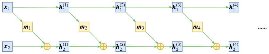Simple coupling leaves part of the variable stuck at the identity, so information isn't fully mixed]

To get a non-trivial transformation, before each additive coupling step we can shuffle or reverse the order of the input dimensions, or simply swap the two parts directly, so that information gets thoroughly mixed, e.g.,

$$\begin{array}{ll}\begin{aligned}&\boldsymbol{h}^{(1)}_{1} = \boldsymbol{x}_{1}\\ &\boldsymbol{h}^{(1)}_{2} = \boldsymbol{x}_{2} + \boldsymbol{m}_1(\boldsymbol{x}_{1})\end{aligned} & \begin{aligned}&\boldsymbol{h}^{(2)}_{1} = \boldsymbol{h}^{(1)}_{1} + \boldsymbol{m}_2\big(\boldsymbol{h}^{(1)}_{2}\big)\\ &\boldsymbol{h}^{(2)}_{2} = \boldsymbol{h}^{(1)}_{2}\end{aligned} & \\ & \\ \begin{aligned}&\boldsymbol{h}^{(3)}_{1} = \boldsymbol{h}^{(2)}_{1}\\ &\boldsymbol{h}^{(3)}_{2} = \boldsymbol{h}^{(2)}_{2} + \boldsymbol{m}_3\big(\boldsymbol{h}^{(2)}_{1}\big)\end{aligned} & \begin{aligned}&\boldsymbol{h}^{(4)}_{1} = \boldsymbol{h}^{(3)}_{1} + \boldsymbol{m}_4\big(\boldsymbol{h}^{(3)}_{2}\big)\\ &\boldsymbol{h}^{(4)}_{2} = \boldsymbol{h}^{(3)}_{2} \end{aligned} & \quad\dots \end{array}\tag{13}$$

as shown below:

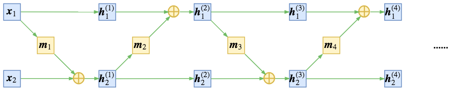Cross-coupling thoroughly mixes information, achieving stronger nonlinearity]

The Scaling Layer

Earlier in this post we already noted that flow is built on invertible transformations, so once the model is trained, we get both a generative model and an encoder model at the same time. But precisely because the transformation is invertible, the random variable $\boldsymbol{z}$ and the input sample $\boldsymbol{x}$ must be the same size. When we specify $\boldsymbol{z}$ to be a Gaussian distribution, it spans the entire $D$-dimensional space, where $D$ is also the size of the input $\boldsymbol{x}$. But even though $\boldsymbol{x}$ has $D$ dimensions, it doesn't necessarily actually span the full $D$-dimensional space. For example, MNIST images have 784 pixels, but some pixels remain zero throughout — in both the training and test sets — which shows that the true dimensionality is far less than 784.

In other words, flow models based on invertible transformations inherently suffer from a fairly serious dimension-wasting problem: the input data clearly doesn't lie on a D-dimensional manifold, yet we're forced to encode it as one — is this even feasible?

To address this, NICE introduces a scaling layer, which applies a scale transformation to each dimension of the final encoded features, i.e., something of the form $\boldsymbol{z} = \boldsymbol{s}\otimes \boldsymbol{h}^{(n)}$, where $\boldsymbol{s} = (\boldsymbol{s}_1,\boldsymbol{s}_2,\dots,\boldsymbol{s}_D)$ is also a parameter vector to be optimized (with all elements non-negative). This $\boldsymbol{s}$ vector identifies how important each dimension is (the smaller it is, the more important that dimension; the larger it is, the less important — approaching negligible), which serves to compress the manifold. Note that the Jacobian determinant of this scaling layer is no longer 1; its Jacobian matrix is easily computed to be diagonal:

$$\left[\frac{\partial \boldsymbol{z}}{\partial \boldsymbol{h}^{(n)}}\right] = \text{diag}\, (\boldsymbol{s})\tag{14}$$

so its determinant is $\prod_i \boldsymbol{s}_i$. According to equation $(6)$, we therefore obtain the log-likelihood

$$\log q(\boldsymbol{x}) \sim -\frac{1}{2}\big\Vert \boldsymbol{s}\otimes \boldsymbol{f} (\boldsymbol{x})\big\Vert^2 + \sum_i \log \boldsymbol{s}_i\tag{15}$$

Why does this scaling layer identify the importance of each feature? Actually, this scaling layer can be described in an even clearer way: initially we set the prior distribution of $\boldsymbol{z}$ to be a standard normal, i.e., with all variances equal to 1. In fact, we can also treat the variance of the prior distribution as a trainable parameter. After training, some variances will be larger and some smaller — the smaller the variance, the smaller the "spread" of that feature. If the variance is 0, that feature is always equal to its mean of 0, and the distribution along that dimension collapses to a single point, which means the manifold has effectively lost one dimension.

Unlike in equation $(4)$, let's write out a normal distribution with variance included:

$$q(\boldsymbol{z}) = \frac{1}{(2\pi)^{D/2}\prod\limits_{i=1}^D \boldsymbol{\sigma}_i}\exp\left(-\frac{1}{2}\sum_{i=1}^D \frac{\boldsymbol{z}_i^2}{\boldsymbol{\sigma}_i^2}\right)\tag{16}$$

Substituting the flow model $\boldsymbol{z}=\boldsymbol{f}(\boldsymbol{x})$ into this expression and taking the logarithm, analogous to equation $(6)$, we get

$$\log q(\boldsymbol{x}) \sim -\frac{1}{2}\sum_{i=1}^D \frac{\boldsymbol{f}_i^2(\boldsymbol{x})}{\boldsymbol{\sigma}_i^2} - \sum_{i=1}^D \log \boldsymbol{\sigma}_i\tag{17}$$

Comparing with equation $(15)$, we see that in fact $\boldsymbol{s}_i=1/\boldsymbol{\sigma}_i$. So the scaling layer is equivalent to treating the variance (standard deviation) of the prior distribution as a trainable parameter — if the variance is small enough, we can consider the manifold represented by that dimension to have collapsed to a point, so the overall manifold dimension decreases by one, implicitly enabling dimensionality reduction.

Feature Disentanglement

When we choose the prior distribution to be a Gaussian with independent components, what benefits does this bring beyond ease of sampling?

In a flow model, $\boldsymbol{f}^{-1}$ is the generative model, used to randomly generate samples, while $\boldsymbol{f}$ is the encoder. But unlike the autoencoders found in ordinary neural networks, which "force a low-dimensional bottleneck to reconstruct high-dimensional data in order to extract useful information," a flow model is fully invertible, so there's no information loss at all. So what value does this encoder provide?

This gets at the question of "what makes a good feature." In everyday life, we often abstract certain dimensions to describe things — "tall/short," "fat/thin," "beautiful/ugly," "rich/poor," and so on. What characterizes these dimensions is: "when we say someone is tall, that doesn't necessarily mean they're fat or thin, nor does it necessarily mean they're rich or poor." That is, there's not much necessary correlation between these features — otherwise the features would be redundant. So, a good feature representation, ideally, should have mutually independent dimensions — this achieves feature disentanglement, so that each dimension carries its own independent meaning.

With this understanding, we can now see the benefit of "choosing the prior distribution to be a Gaussian with independent components": because of this independence, we have good reason to say that when we use $\boldsymbol{f}$ to encode the original features, the resulting encoded feature $\boldsymbol{z}=\boldsymbol{f}(\boldsymbol{x})$ has disentangled dimensions. NICE stands for Non-linear Independent Components Estimation — this is exactly what that name means. Conversely, thanks to the independence of each dimension of $\boldsymbol{z}$, in principle, if we control and vary a single dimension, we can observe how the generated image changes as that dimension changes, thereby discovering what that dimension represents.

Similarly, we can also interpolate (weighted-average) the encodings of two images to obtain generated samples with smooth transitions — something that is fully demonstrated in the later Glow model. However, since we only ran MNIST experiments here, this aspect isn't particularly showcased in this post.

Experiments

Here we reproduce the MNIST experiment from the NICE paper using Keras.

Model Details

Let's first summarize the various components of the NICE model. NICE is a type of flow model, composed of multiple additive coupling layers, each taking the form of $(7)$, with inverse given by $(9)$. Before each coupling, the input dimensions need to be reversed so that information is thoroughly mixed. The final layer needs an added scaling layer, and the final loss is the negative of equation $(15)$.

Each additive coupling layer needs to split the input into two parts. NICE uses an interleaved partition, i.e., the even-indexed entries form the first part and the odd-indexed entries form the second part, and each $\boldsymbol{m}(\boldsymbol{x})$ is simply implemented as a multi-layer fully-connected network (5 hidden layers, 1000 units per layer, ReLU activation). In NICE, a total of 4 additive coupling layers are chained together.

For the input, we compress the original 0–255 pixel values down into the 0–1 range (by simply dividing by 255), and then add uniform noise $[-0.01, 0]$ to the input. Adding noise effectively helps prevent overfitting and improves the quality of generated images. It can also be seen as a measure to mitigate the dimension-wasting problem, since MNIST images can't actually fill up all 784 dimensions in reality — but once you factor in the noise, the effective dimensionality increases.

Readers might wonder: why is the noise interval $[-0.01, 0]$, and not $[0, 0.01]$ or $[-0.005, 0.005]$? In fact, judging by the loss, various kinds of noise all give roughly the same result (including swapping the uniform distribution for a Gaussian). But once noise is added, in theory the generated images will also carry noise, which isn't what we want. By adding negative-valued noise, the pixel values of the final generated images end up shifted slightly toward the negative range, which means I can simply use a clip operation to remove some of that noise. This is just a small (and not particularly important) trick specific to MNIST.

Reference Code

Here is my reference implementation in Keras:

https://github.com/bojone/flow/blob/master/nice.py]

In my experiments, the model reaches optimal quality within 20 epochs, taking about 11 seconds per epoch (on a GTX 1070), with a final loss of around -2200.

Compared to the original paper's implementation, I made a few changes here. For the additive coupling layer, I used equation $(9)$ for the forward pass and equation $(7)$ for its inverse. Since $\boldsymbol{m}(\boldsymbol{x})$ uses ReLU activation, and we know ReLU outputs are non-negative, these two choices do make a bit of a difference. Since the forward direction is the encoder and the inverse direction is the generator, choosing equation $(7)$ as the inverse means the generative model is biased toward producing positive values, which matches what we want to generate, since we need to produce images with pixel values in the 0–1 range.

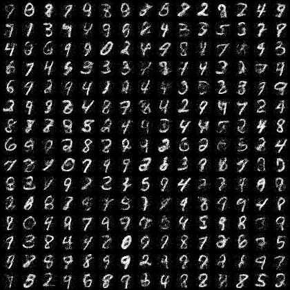Digit samples generated by the NICE model (trained without noise)]
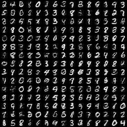Digit samples generated by the NICE model (trained with negative noise)]

Annealing Parameter

Although we ultimately want to sample random numbers from a standard normal distribution to generate samples, in practice, for a trained model, the ideal sampling variance isn't necessarily 1 — it fluctuates around 1, and is generally a bit smaller than 1. We call the standard deviation of the final sampling normal distribution the annealing parameter. In the reference implementation above, for instance, we chose an annealing parameter of 0.75, which by visual inspection produced the best-quality generated model.

Summary

The NICE model is actually fairly large: following the setup described above, the total parameter count is roughly $4 \times 5 \times 1000^2 = 2\times 10^7$ — that is, twenty million parameters just to train a generative model for MNIST, which is honestly a bit excessive.

Overall, NICE is still fairly simple and brute-force: the additive coupling itself is quite simple, and the $\boldsymbol{m}$ portion of the model just uses large fully-connected layers, without incorporating tricks like convolutions. So there's still plenty of room for exploration — Real NVP and Glow are two improved versions built on this foundation, and we'll get to their stories later on.