The Reversible ResNet in the Flow Series: An Extreme Aesthetic of Brute Force
Today we're going to introduce a rather "brutal" model: the invertible ResNet.
Why would one call a model "brutal"? Because it genuinely is: it brings together a whole arsenal of mathematical tricks to forcibly (under certain constraints) turn an ordinary ResNet into an invertible one!
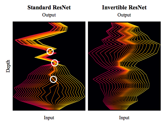 Comparison of a standard ResNet and an invertible ResNet. The invertible ResNet allows information to flow losslessly and reversibly, while the standard ResNet exhibits a "collapse" at some point.
The model comes from Invertible Residual Networks, which was also previously reported on by Jiqizhixin. In this post, we'll take a simple look at its principles and content.
A Few Words on Invertible Models
Why study invertible ResNet models? What are the benefits? Hasn't anyone studied this before?
The Benefits of Invertibility
What does invertibility mean?
It means the model is information-lossless, which suggests it might make a better classification network, and it means we can directly use maximum likelihood to build a generative model. Moreover, thanks to the powerful capacity of ResNet, it might even outperform the earlier Glow model. In short: if a model is invertible, if the cost of invertibility is low, and if its fitting capacity is strong, then it has a very wide range of uses (classification, density estimation, generation tasks, and so on). More
The invertible ResNet introduced in this post basically satisfies all these requirements: making it invertible is relatively simple, and it barely changes ResNet's fitting capacity at all. For this reason, I think it deserves to be called a "beautiful" model.
The Limitations of Earlier Models
Invertible models have a long research history — they're known as "flow-based models," with representative models including NICE, RealNVP, and Glow, all of which I've written about before, along with a few autoregressive flow models. Besides being used as generative models, invertible models have also been studied for classification tasks, with RevNet and i-RevNet as representative works.
These flow models basically all share the same design philosophy: through clever design, the inverse transform of each layer is made simple, and the Jacobian matrix is made triangular so that the Jacobian determinant is easy to compute. Such models are theoretically elegant and beautiful, but they have one serious drawback: because the inverse transform must remain simple and the Jacobian determinant must remain easy to compute, the nonlinear transformation capacity of each layer is very weak. In fact, in a model like Glow, only half of the variables are transformed at each layer, so in order to guarantee sufficient fitting capacity, the model has to be stacked extremely deep (for example, for 256×256 face generation, Glow stacks around 600 convolutional layers, with about 200 million parameters), which is computationally very expensive.
Head-On Against the Residual Model
This time, the invertible ResNet takes a different approach from previous flow models: it simply adds some constraints on top of an ordinary ResNet structure to make the model invertible, while essentially preserving ResNet's basic structure and most of its fitting capacity. This means that our accumulated design experience with ResNets largely still applies, and the model no longer needs to stack convolutions as desperately as Glow does.
Of course, there's a price to pay: without any special design tricks, we need fairly brute-force methods to obtain the inverse function and the Jacobian determinant. So this invertible ResNet is beautiful, but also brutal — it truly deserves the title of "extreme aesthetic of brute force."
The "Three Essentials" of Invertibility
The basic building block of a ResNet model is
\begin{equation}y = x + g(x)\triangleq F(x)\label{eq:resnet}\end{equation}
That is, instead of using a neural network to directly fit $y$, we now use a neural network to fit $y-x$, where $x,y$ are all vectors (tensors). The benefit of this is that gradients don't vanish as easily, deep networks can be trained, information can flow through multiple channels, and so on. Invertibility means that $x+g(x)$ is a bijection — that is, each $x$ corresponds to exactly one $y$, and vice versa, so that in theory we can solve for the inverse function $x=h(y)$.
I won't dwell on the background, but let me clarify one point: the generalized ResNet that we typically use in classification problems allows the dimensionality to change via $1\times 1$ convolutions, but the ResNet discussed here refers to a ResNet that does not change dimensionality — that is, the size of $x,y$ stays the same throughout.
For a model that claims to be "invertible," there are three questions it must answer:
1. When is it invertible?
2. What is the inverse function?
3. How do we compute the Jacobian determinant?
In terms of difficulty, these three questions build progressively on one another. Of course, if you only care about classification, then satisfying the first point is enough; if you care about reconstructing images, you'll need the second point too; and if you want to train a generative model with maximum likelihood, as Glow does, you'll need the third point as well.
Below, following the reasoning of the original paper, we tackle these three questions one by one (three "hard dishes") — a feast of brute force.
When Is It Invertible?
The first hard dish is relatively easier to chew among the three, though of course "relatively" is the operative word — it still draws on some basic knowledge of functional analysis. (Dear reader, don't run away just yet!)
Since $\eqref{eq:resnet}$ is the basic building block of the ResNet, we just need to ensure that each block is invertible. A sufficient condition for $\eqref{eq:resnet}$ to be invertible is:
\begin{equation}\text{Lip}(g) < 1\end{equation}
where
\begin{equation}\text{Lip}(g) \triangleq \max_{x_1\neq x_2}\frac{\Vert g(x_1) - g(x_2)\Vert_2}{\Vert x_1 - x_2\Vert_2}\end{equation}
is the Lipschitz norm of the function $g$. In other words, if the Lipschitz norm of $g$ is less than 1, then $\eqref{eq:resnet}$ is guaranteed to be invertible.
So when is the Lipschitz norm of $g$ less than 1? Since $g$ is a neural network — convolutional or fully connected, it doesn't matter — a neural network is built from a combination of matrix operations and activation functions, taking the representative form
\begin{equation}Activation(Wx+b)\end{equation}
Then, by the chain rule, a sufficient condition for "the Lipschitz norm of $g$ being less than 1" is that "the Lipschitz norm of $Activation$ is at most 1" and "the Lipschitz norm of $Wx+b$ is less than 1." Since $Activation$ is just a scalar function, "Lipschitz norm at most 1" simply means its derivative doesn't exceed 1, which holds for all the activation functions we commonly use (sigmoid, tanh, ReLU, ELU, swish, etc.), so we don't need to worry about that. As for "the Lipschitz norm of $Wx+b$ being less than 1," this means the Lipschitz norm of the matrix $W$ must be less than 1.
The Lipschitz norm of the matrix $W$ is actually its "spectral norm," which we can write as $\text{Lip}(W)$ or $\Vert W\Vert_2$. Where have we seen the spectral norm of a matrix before? It came up in our discussion of Lipschitz constraints in Lipschitz Constraints in Deep Learning: Generalization and Generative Models. Combining the two, we arrive at the conclusion:
By applying spectral normalization to all the kernel weights $W$ of model $g$, and then multiplying by a coefficient $c$ between 0 and 1 (i.e., $W\leftarrow c W / \Vert W\Vert_2$), we can make $x+g(x)$ invertible.
What Is the Inverse Function?
Why does this make the model invertible? The proof directly answers the second question too — that is, we can directly derive the inverse function, and in doing so we'll see exactly under what conditions invertibility holds.
Suppose $y=x+g(x)$ is invertible; then we need a way of computing the inverse function $x=h(y)$, which really amounts to solving a system of nonlinear equations. For simplicity, consider the iteration
\begin{equation}x_{n+1}=y - g(x_n)\label{eq:nidiedai}\end{equation}
Clearly, the iterative sequence $\{x_n\}$ depends on $y$, and once $\{x_n\}$ converges to some fixed function
\begin{equation}\lim_{n\to\infty} x_n(y) = \hat{h}(y)\end{equation}
we then have $\hat{h}(y)=y-g\left(\hat{h}(y)\right)$, which means $\hat{h}(y)$ is exactly the $x=h(y)$ we're looking for.
In other words, if the iteration $\eqref{eq:nidiedai}$ converges, the result of convergence is precisely the inverse function of $x+g(x)$. So all we need to do is figure out when $\eqref{eq:nidiedai}$ converges. This is where the earlier condition $\text{Lip}(g) < 1$ comes into play — we have
\begin{equation}\forall x_1,x_2,\quad\Vert g(x_1) - g(x_2)\Vert_2\leq \text{Lip}(g)\Vert x_1 - x_2\Vert_2\end{equation}
and therefore
\begin{equation}\begin{aligned}\Vert x_{n+1} - x_{n}\Vert_2&=\Vert g(x_{n}) - g(x_{n-1})\Vert_2\\ &\leq \text{Lip}(g)\Vert x_{n} - x_{n-1}\Vert_2\\ & = \text{Lip}(g)\Vert g(x_{n-1}) - g(x_{n-2})\Vert_2\\ &\leq \text{Lip}(g)^2\Vert x_{n-1} - x_{n-2}\Vert_2\\ &\dots\\ &\leq \text{Lip}(g)^n\Vert x_{1} - x_{0}\Vert_2\\ \end{aligned}\end{equation}
We can see that a sufficient condition for $\Vert x_{n+1} - x_{n}\Vert_2\to 0$ is $\text{Lip}(g) < 1$.
Note: Merely showing $\Vert x_{n+1} - x_{n}\Vert_2\to 0$ does not by itself establish that the sequence $\{x_n\}$ converges — for instance, a sequence like $\{\ln n\}$ also satisfies this condition yet diverges. So, to properly prove convergence of $\{x_n\}$ under the condition $\text{Lip}(g) < 1$, some extra work is needed. But this is a fairly mathematical detour, and since some readers may not be interested, I've put it in a note.
For any positive integer $k$, let's further examine $\Vert x_{n+k} - x_{n}\Vert_2$:
\begin{equation}\begin{aligned}\Vert x_{n+k} - x_{n}\Vert_2&\leq\Vert x_{n+k} - x_{n+k-1}\Vert_2+\dots+\Vert x_{n+2} - x_{n+1}\Vert_2+\Vert x_{n+1} - x_{n}\Vert_2\\ > &\leq \left(\text{Lip}(g)^{n+k-1}+\dots+\text{Lip}(g)^{n+1}+\text{Lip}(g)^{n}\right)\Vert x_{1} - x_{0}\Vert_2\\ > & = \frac{1 - \text{Lip}(g)^k}{1 - \text{Lip}(g)}\cdot\text{Lip}(g)^{n}\Vert x_{1} - x_{0}\Vert_2\\ > & \leq \frac{\text{Lip}(g)^n}{1 - \text{Lip}(g)}\Vert x_{1} - x_{0}\Vert_2 > \end{aligned}\label{eq:cauchy}\end{equation}
We obtain an upper bound on $\Vert x_{n+k} - x_{n}\Vert_2$ that depends only on $n$, and which can be made arbitrarily small. That is, for any $\varepsilon > 0$, we can find an $n$ such that for any positive integer $k$, we have $\Vert x_{n+k} - x_{n}\Vert_2 < \varepsilon$. Such a sequence is called a Cauchy sequence, and it must converge. This finally establishes the convergence of $\{x_n\}$.
Incidentally, if in $\eqref{eq:cauchy}$ we take $k\to\infty$, we obtain:
\begin{equation}\left\Vert x^* - x_{n}\right\Vert_2 \leq \frac{\text{Lip}(g)^n}{1 - \text{Lip}(g)}\Vert x_{1} - x_{0}\Vert_2\end{equation}
That is, the convergence speed of this iterative algorithm is proportional to $\text{Lip}(g)^n$, so naturally the smaller $\text{Lip}(g)$ is, the faster the convergence — but the smaller $\text{Lip}(g)$ is, the weaker the model's fitting capacity becomes. In the original paper, its range is chosen to be roughly 0.5 to 0.9.
Put more grandly, this is exactly the Banach fixed-point theorem from functional analysis, also known as the contraction mapping theorem (since $\text{Lip}(g)$ is less than 1, $g$ is called a contraction mapping).
With this, we've now answered why $\text{Lip}(g) < 1$ guarantees that $x+g(x)$ is invertible, and we've also given a method for computing the inverse function — namely, iterating $\eqref{eq:nidiedai}$ to sufficient precision:
Once normalization has been applied so that $x+g(x)$ is invertible, its inverse function is the fixed point of $x_{n+1}=y - g(x_n)$. In practice, one simply iterates a certain number of steps until the desired precision is reached.
At last, we've chewed through the second hard dish.
How Do We Compute the Jacobian Determinant?
Now we come to the most "hardcore" of the three questions: how do we compute the Jacobian determinant? To solve it, the authors bring together tools from mathematical analysis, matrix theory, probability theory, and statistical sampling — truly the most brutal, hardest dish of all.
First, why do we need to compute the Jacobian determinant at all? As mentioned earlier, this is only necessary when building a generative model; for details, please refer to the earliest post on this site about flow models, NICE: The Basic Concepts and Implementation of Flow Models. Next, recall that the Jacobian determinant is the determinant of the Jacobian matrix, so we first need to compute the Jacobian matrix:
\begin{equation}J_F\triangleq \frac{\partial}{\partial x}(x+g(x))= I + \frac{\partial g}{\partial x}\triangleq I + J_g\end{equation}
Just a reminder — although I've been lazy and not used bold notation, the output $g$ here is a vector, $x$ is also a vector, and $\partial g / \partial x$ is essentially the pairwise partial derivatives between input and output components, giving a matrix (the Jacobian matrix).
Then, the Jacobian determinant is $\det(J_F)=\det (I+J_g)$, but in fact, when building generative models, what we really need to compute is "the logarithm of the absolute value of the Jacobian determinant," i.e.,
\begin{equation}\ln |\det(J_F)| = \ln |\det(I + J_g)|\equiv \ln \det(I + J_g)\end{equation}
The final equality holds because $\det(I + J_g)$ is always positive, so we can drop the absolute value. This can be proven, but it's a technical detail we won't dwell on here — interested readers can consult the references the authors provide.
So what next? Should we just compute the Jacobian determinant directly from its definition? No — that would be far too computationally expensive, and during backpropagation we'd also need to differentiate the determinant, which would be even more complicated. The authors came up with a laborious but effective solution, using the identity (see Appreciating the Identity det(exp(A)) = exp(Tr(A))):
\begin{equation}\ln\det(\boldsymbol{B}) = \text{Tr}(\ln (\boldsymbol{B}))\end{equation}
we obtain
\begin{equation}\ln\det(I + J_g) = \text{Tr}(\ln (I+J_g))\end{equation}
If we can compute $\ln (I+J_g)$, we can then just take its trace (the sum of the diagonal elements). How do we compute $\ln (I+J_g)$? Again referring to Appreciating the Identity det(exp(A)) = exp(Tr(A)), we simply expand it brute-force:
\begin{equation}\ln (I + J_g) = \sum_{n=1}^{\infty}(-1)^{n-1}\frac{J_g^n}{n}\label{eq:duishujishu}\end{equation}
Note that this series converges under the condition $\Vert J_g\Vert_2 < 1$, which precisely corresponds to $\text{Lip}(g) < 1$ — exactly the constraint of the invertible ResNet. Everything is perfectly self-consistent.
Now $\ln (I + J_g)$ has become an infinite series; if we truncate it at $n$ terms, the error is proportional to $\text{Lip}(g)^n$, so we need to look at $\text{Lip}(g)$ to decide how many terms to keep. This lets us write
\begin{equation}\text{Tr}(\ln (I + J_g)) = \sum_{n=1}^{N}(-1)^{n-1}\frac{\text{Tr}(J_g^n)}{n}+\mathcal{O}\left(\text{Lip}(g)^N\right)\label{eq:det2tr}\end{equation}
Is the problem solved? Not quite — the expression above requires us to compute $J_g^n$, and note that $J_g$ is a matrix, so we'd need to compute the $n$-th power of a matrix (imagine the workload of just computing two matrix multiplications). So the authors thought:
Since we've exhausted the tools of analysis, let's bring in probability and statistics.
Suppose $p(u)$ is a multivariate probability distribution with zero mean and identity covariance (clearly the standard normal distribution satisfies this), then for any matrix $A$, we have
\begin{equation}\text{Tr}(A)=\mathbb{E}_{u\sim p(u)}\big[u^{\top}Au\big]\end{equation}
Using the property "zero mean, identity covariance," this identity can be proven directly from the definition without much difficulty. Then, the authors proposed a method that seems "both shameless and reasonable": for each iteration, we just randomly draw a single vector $u$ from $p(u)$, and treat $u^{\top}Au$ as if it were $\text{Tr}(A)$, i.e.,
\begin{equation}\text{Tr}(\ln (I + J_g)) \approx \sum_{n=1}^{N}(-1)^{n-1}\frac{u^{\top} J_g^n u}{n},\quad u\sim p(u)\label{eq:tr-caiyang}\end{equation}
Readers might object here — aren't we supposed to average over all possible vectors? Can we really get away with just picking one at random? As it turns out, yes, and here's why:
1. Our optimization is already based on stochastic gradient descent, which inherently carries error; randomly picking just one vector introduces error too, but since we re-sample a different $u_1,u_2$ at every iteration, the errors tend to cancel out to some extent over training;
2. More importantly, computing the log-determinant of the Jacobian only serves as an auxiliary loss term to prevent the model from collapsing. Put simply, it functions as a regularization term — and since it's just a regularization term, a bit of error here is perfectly tolerable.
So, the computation of $\text{Tr}(J_g^n)$ is resolved by the authors with this crude (yet effective) scheme. Note that
\begin{equation}u^{\top} J_g^n u=u^{\top} J_g(\dots(J_g(J_g u)))\end{equation}
so there's no need to explicitly compute $J_g^n$; instead, at each step we only need to compute the product of a matrix and a vector, and the computation at each step can be reused, which greatly reduces the overall computational cost.
So, to summarize:
By expanding the Jacobian matrix as a logarithmic series $\eqref{eq:duishujishu}$, converting the determinant computation into a trace computation $\eqref{eq:det2tr}$, and exploiting probabilistic sampling $\eqref{eq:tr-caiyang}$, we can compute the Jacobian determinant in the most efficient way possible.
A Look at the Experimental Results
Honestly, I was initially drawn in by the beautiful idea of the "invertible ResNet," but by this point, I have to admit I've wimped out a bit myself — this thing truly earns the description "wrestling ResNet into submission." I originally wanted to try implementing something like an MNIST generation experiment to play around with, but once I confirmed just how many tricks and just how much brute force were involved, I gave up on that idea.
So instead, let's just look at the experimental results from the original paper.
Toy Dataset
First, a synthetic toy dataset — that is, some artificially constructed points with a certain regular structure, which we then try to fit with a generative model. This is a common kind of experiment in GAN research as well. As the figure below shows, the invertible ResNet performs much better than Glow. Fundamentally, I think this is because the invertible ResNet is a very symmetric model with little inherent bias, whereas Glow is biased: it requires us to shuffle the input in some way and then split it in half, applying different operations to each half — and this asymmetry is exactly the source of the bias.
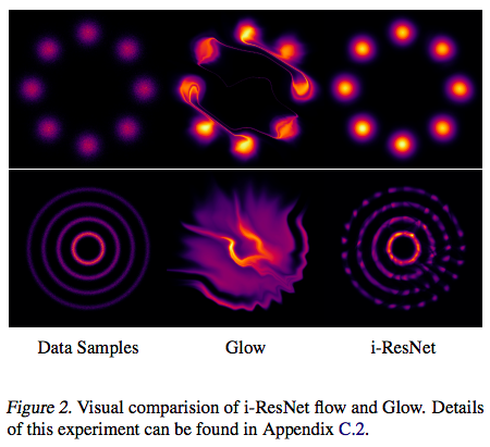 Invertible ResNet experiment: toy dataset
Classification Experiments
As mentioned at the outset, since this is a variant of ResNet, its most basic use case is classification. The table below shows that using the invertible ResNet for classification also achieves strong results — the presence of the Lipschitz constraint doesn't noticeably hurt classification performance ($c$ in the table refers to $\text{Lip}(g)$).
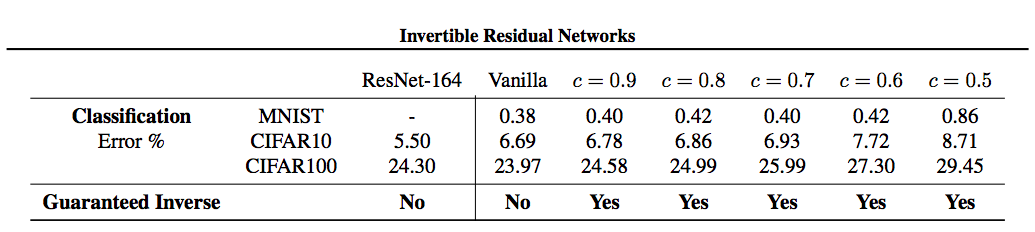 Invertible ResNet experiment: classification results
Generative Model Experiments
In truth, flow-based models are still far behind GANs when it comes to generating complex images, but quantitative comparisons among flow models themselves are perfectly valid. The figure below shows that the invertible ResNet also performs excellently as a flow-based generative model.
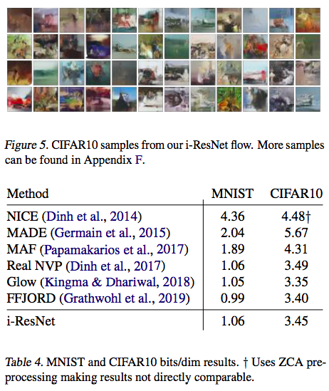 Invertible ResNet experiment: generative model results
Time to Wrap Up
Forcibly wrestling ResNet into being invertible really is grueling work — even just explaining it left me exhausted, so I have great respect for the mathematical rigor of the authors. Of course, in the end, the authors did succeed, and I imagine the joy of that success must have been substantial. Overall, the whole piece of work is brutal in method, but on closer reflection there's nothing forced or awkward about it — if anything, there's a natural, cohesive beauty to it, rather than a mere pile-up of mathematical formulas.
The one issue is that the entire "brute-force" pipeline is still quite complex, so widespread adoption really requires a good, clean implementation — and that's often exactly what discourages people from trying. There's another issue too: since flow models must preserve invertibility, they naturally cannot reduce dimensionality, but without dimensionality reduction, the computational cost is inevitably large. This is something of a contradiction.
One intriguing idea is this: for the case of dimensionality reduction, could we construct something like a matrix "pseudo-inverse" analog to achieve an effect similar to the invertible ResNet? Even non-square matrices can be assigned a kind of determinant (see Revisiting the Determinant of Non-Square Matrices), so it seems plausible that dimension-reducing transformations could also be given some analogue of a log-Jacobian-determinant. It looks like quite a few of these ideas could potentially be generalized.
Where will the flow model line of research head next? Let's wait and see.
Translated automatically with claude-sonnet-5; all equations are reproduced verbatim from the source. Copyright remains with the original author.