Can Attention Mechanisms Really "Concentrate Attention"?

注意力机制真的可以“集中注意力”吗？ 苏剑林 · 2023-12-12 · Machine Learning entropy sparse attention rank

In earlier posts such as 《Transformer Upgrade Path: 3. From Performer to Linear Attention》 and 《Why Are Today's LLMs All Decoder-Only Architectures?》, we examined attention mechanisms from the perspective of the "rank" of the attention matrix, and once concluded that the key reason linear attention underperforms standard attention is precisely the "low-rank bottleneck." However, while this explanation may hold for bidirectional Encoder models, it is hard to apply to unidirectional Decoder models, since the upper-triangular part of a Decoder's attention matrix is masked out, leaving a lower-triangular matrix that is necessarily full rank. And if it's already full rank, then the low-rank bottleneck issue seemingly no longer applies.

So the "low-rank bottleneck" cannot fully explain the capability gap of linear attention. In this post, I try to seek an explanation from a different angle. Simply put, compared with standard attention, linear attention finds it harder to "concentrate attention," making it difficult to accurately pinpoint key tokens — and this is probably the main reason its performance falls somewhat short.

Degree of Sparsity

In the post 《Viewing the Scale Operation in Attention Through the Lens of Entropy Invariance》, we examined the attention mechanism from the angle of "concentration of attention," using information entropy as a measure of "degree of concentration": the lower the entropy, the more likely attention is concentrated on a particular token.

However, for general attention mechanisms, the attention matrix may be unnormalized — for example, the GAU module introduced in 《FLASH: Perhaps the Most Interesting Efficient Transformer Design in Recent Times》, and the $l_2$-normalized attention introduced in 《A Theoretical Flaw in Relative Positional Encoding Transformers and a Countermeasure》. Indeed, from the even more general perspective of Non-Local Neural Networks, the attention matrix need not even be non-negative. Such unnormalized, or even non-negative-violating, attention matrices are naturally not amenable to information entropy, since entropy is defined for probability distributions.

To address this, we consider the sparsity metric of the $l_1/l_2$ form introduced in 《How to Measure the Sparsity of Data?》:

\begin{equation}S(x) = \frac{\mathbb{E}[|x|]}{\sqrt{\mathbb{E}[x^2]}}\end{equation}

This metric is similar to information entropy: a smaller $S(x)$ means the corresponding random vector is sparser, and sparser means it's more likely that "one dominates all," corresponding to a one-hot distribution in probability terms. Unlike entropy, though, it applies to general random variables or vectors.

A Simplified Form

For the attention mechanism, let us write $\boldsymbol{a} = (a_1,a_2,\cdots,a_n)$, where $a_j \propto f(\boldsymbol{q}\cdot\boldsymbol{k}_j)$, so that

\begin{equation}S(\boldsymbol{a}) = \frac{\mathbb{E}_{\boldsymbol{k}}[|f(\boldsymbol{q}\cdot\boldsymbol{k})|]}{\sqrt{\mathbb{E}_{\boldsymbol{k}}[f^2(\boldsymbol{q}\cdot\boldsymbol{k})]}}\end{equation}

In what follows we always consider the limit $n\to\infty$. Assume $\boldsymbol{k}\sim\mathcal{N}(\boldsymbol{\mu},\sigma^2\boldsymbol{I})$, so we can set $\boldsymbol{k} = \boldsymbol{\mu} + \sigma \boldsymbol{\varepsilon}$, where $\boldsymbol{\varepsilon}\sim\mathcal{N}(\boldsymbol{0},\boldsymbol{I})$, giving

\begin{equation}S(\boldsymbol{a}) = \frac{\mathbb{E}_{\boldsymbol{\varepsilon}}[|f(\boldsymbol{q}\cdot\boldsymbol{\mu} + \sigma\boldsymbol{q}\cdot\boldsymbol{\varepsilon})|]}{\sqrt{\mathbb{E}_{\boldsymbol{\varepsilon}}[f^2(\boldsymbol{q}\cdot\boldsymbol{\mu} + \sigma\boldsymbol{q}\cdot\boldsymbol{\varepsilon})]}}\end{equation}

Note that the distribution $\mathcal{N}(\boldsymbol{0},\boldsymbol{I})$ followed by $\boldsymbol{\varepsilon}$ is isotropic. As in the simplification approach derived in 《The Angle Distribution Between Two Random Vectors in n-Dimensional Space》, because of isotropy, the expectation involving $\boldsymbol{q}\cdot\boldsymbol{\varepsilon}$ depends only on the magnitude of $\boldsymbol{q}$ and not on its direction. So we can simplify $\boldsymbol{q}$ to $(\Vert\boldsymbol{q}\Vert,0,0,\cdots,0)$, and the expectation over $\boldsymbol{\varepsilon}$ then simplifies to

\begin{equation}S(\boldsymbol{a}) = \frac{\mathbb{E}_{\varepsilon}[|f(\boldsymbol{q}\cdot\boldsymbol{\mu} + \sigma\Vert\boldsymbol{q}\Vert\varepsilon)|]}{\sqrt{\mathbb{E}_{\varepsilon}[f^2(\boldsymbol{q}\cdot\boldsymbol{\mu} + \sigma\Vert\boldsymbol{q}\Vert\varepsilon)]}}\end{equation}

where $\varepsilon\sim\mathcal{N}(0,1)$ is a random scalar.

Two Examples

We can now compute and compare a few common choices of $f$. The most commonly used attention mechanism today is $f=\exp$, in which case the expectation reduces to an ordinary one-dimensional Gaussian integral, and we can readily compute

\begin{equation}S(\boldsymbol{a}) = \exp\left(-\frac{1}{2}\sigma^2\Vert\boldsymbol{q}\Vert^2\right)\end{equation}

When $\sigma\to\infty$ or $\Vert\boldsymbol{q}\Vert\to\infty$, we always have $S(\boldsymbol{a})\to 0$, meaning that in theory standard attention can indeed "concentrate attention" to an arbitrary degree of sparsity. This also tells us how to make attention more concentrated: increase the magnitude of $\boldsymbol{q}$, or increase the variance across the various $\boldsymbol{k}$ — in other words, widen the gap between the $\boldsymbol{k}$.

Another example is GAU (Gated Attention Unit), a personal favorite of mine. When it was originally proposed it used $f=\text{relu}^2$ (though later, when I used it myself, I reverted to Softmax — see 《FLASH: Perhaps the Most Interesting Efficient Transformer Design in Recent Times》 and 《I Heard Attention Pairs Better with Softmax～》). In this case the integral isn't as simple as with $f=\exp$, but it can still be brute-forced with Mathematica, giving

\begin{equation}S(\boldsymbol{a}) =\frac{e^{-\frac{\beta ^2}{2 \gamma ^2}} \left(\sqrt{2} \beta \gamma +\sqrt{\pi } e^{\frac{\beta ^2}{2 \gamma ^2}} \left(\beta ^2+\gamma ^2\right) \left(\text{erf}\left(\frac{\beta }{\sqrt{2} \gamma }\right)+1\right)\right)}{\sqrt[4]{\pi } \sqrt{2 \sqrt{2} \beta \gamma e^{-\frac{\beta ^2}{2 \gamma ^2}} \left(\beta ^2+5 \gamma ^2\right)+2 \sqrt{\pi } \left(\beta ^4+6 \beta ^2 \gamma ^2+3 \gamma ^4\right) \left(\text{erf}\left(\frac{\beta }{\sqrt{2} \gamma }\right)+1\right)}}\end{equation}

where $\beta = \boldsymbol{q}\cdot\boldsymbol{\mu}, \gamma = \sigma\Vert\boldsymbol{q}\Vert$. The expression looks fearsome, but no matter — let's just plot it:

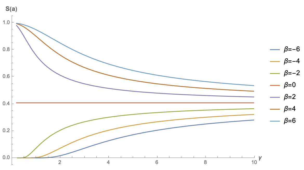Sparsity curve for relu² attention

As we can see, only when $\beta < 0$ does the sparsity of the original GAU have a chance of approaching 0. This is also intuitive: when the bias term is less than 0, there's more opportunity for the result of $\text{relu}$ to be 0, thereby achieving sparsity. This result also shows that, unlike the standard attention with $f=\exp$, the bias term in $\boldsymbol{k}$ can have a positive effect on GAU with $f=\text{relu}^2$.

Minimal Linear Attention

Next, let's look at the simplest possible example: without adding $f$, or equivalently, $f=\text{identical}$. This corresponds to the simplest form of linear attention, and again we can brute-force the calculation with Mathematica to get:

\begin{equation}S(\boldsymbol{a}) =\frac{\sqrt{\frac{2}{\pi }} \gamma e^{-\frac{\beta ^2}{2 \gamma ^2}}+\beta \text{erf}\left(\frac{\beta }{\sqrt{2} \gamma }\right)}{\sqrt{\beta ^2+\gamma ^2}}\end{equation}

Below are the function plots for a few different values of $\beta$:

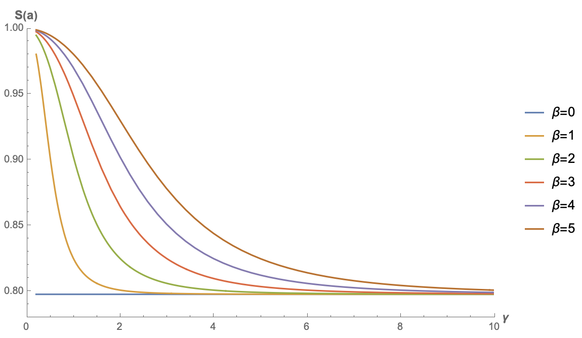Sparsity curve for minimal linear attention

Note that $S(\boldsymbol{a})$ here is an even function of $\beta$ (readers might try proving this themselves), so the plot for $\beta < 0$ is identical to that of its negative, and hence the figure above only shows the results for $\beta \geq 0$. As the figure shows, linear attention without any activation function cannot bring the sparsity close to 0 — instead, there's a fairly high lower bound. This means that when the input sequence is long enough, this kind of linear attention has no way to "concentrate attention" on key positions.

General Linear Attention

From 《Exploring Linear Attention: Must Attention Have a Softmax?》, we know that the general form of linear attention is $a_j \propto g(\boldsymbol{q})\cdot h(\boldsymbol{k}_j)$, where $g,h$ is an activation function with non-negative range. Let us write $\tilde{\boldsymbol{q}}=g(\boldsymbol{q}),\tilde{\boldsymbol{k}}=h(\boldsymbol{k})$, so that $a_j\propto \tilde{\boldsymbol{q}}^{\scriptscriptstyle\top}\tilde{\boldsymbol{k}}$, and we can derive

\begin{equation}S(\boldsymbol{a}) = \frac{\mathbb{E}_{\boldsymbol{\varepsilon}}\left[\tilde{\boldsymbol{q}}^{\scriptscriptstyle\top}\tilde{\boldsymbol{k}}\right]}{\sqrt{\mathbb{E}_{\boldsymbol{\varepsilon}}\left[\tilde{\boldsymbol{q}}^{\scriptscriptstyle\top}\tilde{\boldsymbol{k}}\tilde{\boldsymbol{k}}^{\scriptscriptstyle\top}\tilde{\boldsymbol{q}}\right]}} = \frac{\tilde{\boldsymbol{q}}^{\scriptscriptstyle\top}\mathbb{E}_{\boldsymbol{\varepsilon}}\left[\tilde{\boldsymbol{k}}\right]}{\sqrt{\tilde{\boldsymbol{q}}^{\scriptscriptstyle\top}\mathbb{E}_{\boldsymbol{\varepsilon}}\left[\tilde{\boldsymbol{k}}\tilde{\boldsymbol{k}}^{\scriptscriptstyle\top}\right]\tilde{\boldsymbol{q}}}} = \frac{\tilde{\boldsymbol{q}}^{\scriptscriptstyle\top}\tilde{\boldsymbol{\mu}}}{\sqrt{\tilde{\boldsymbol{q}}^{\scriptscriptstyle\top}\left[\tilde{\boldsymbol{\mu}}\tilde{\boldsymbol{\mu}}^{\scriptscriptstyle\top} + \tilde{\boldsymbol{\Sigma}}\right]\tilde{\boldsymbol{q}}}} = \frac{1}{\sqrt{1 + \frac{\tilde{\boldsymbol{q}}^{\scriptscriptstyle\top}\tilde{\boldsymbol{\Sigma}}\tilde{\boldsymbol{q}}}{(\tilde{\boldsymbol{q}}^{\scriptscriptstyle\top}\tilde{\boldsymbol{\mu}})^2}}}\end{equation}

This is a general result for non-negative-type linear attention, with no approximations made so far, where $\tilde{\boldsymbol{\mu}},\tilde{\boldsymbol{\Sigma}}$ are respectively the mean vector and covariance matrix of the $\tilde{\boldsymbol{k}}$ sequence.

From this result we see that non-negative-type linear attention can also become arbitrarily sparse (i.e., $S(\boldsymbol{a})\to 0$), as long as the mean tends to 0, or the covariance tends toward $\infty$ — that is, as long as the signal-to-noise ratio of the $\tilde{\boldsymbol{k}}$ sequence is as small as possible. However, the $\tilde{\boldsymbol{k}}$ sequence is a sequence of non-negative vectors, and a non-negative sequence with a small signal-to-noise ratio means that most elements of the sequence are close to each other, so such a sequence can only express limited information. This also means that linear attention can typically only represent the importance of absolute position (e.g., an attention matrix where an entire column is all 1s), rather than adequately expressing the importance of relative position — which is essentially another manifestation of linear attention's low-rank bottleneck.

To get a more concrete sense of how $S(\boldsymbol{a})$ changes, let's assume the simplest scenario: each component of $\tilde{\boldsymbol{k}}$ is i.i.d., in which case the mean vector simplifies to $\tilde{\mu}\boldsymbol{1}$ and the covariance matrix simplifies to $\tilde{\sigma}^2\boldsymbol{I}$, so the formula for $S(\boldsymbol{a})$ further simplifies to

\begin{equation}S(\boldsymbol{a}) = \frac{1}{\sqrt{1 + \left(\frac{\tilde{\sigma}}{\tilde{\mu}}\frac{\Vert\tilde{\boldsymbol{q}}\Vert_2}{\Vert\tilde{\boldsymbol{q}}\Vert_1}\right)^2}}\end{equation}

This result is much more intuitive to look at. To make linear attention sparser, one direction is to increase $\frac{\tilde{\sigma}}{\tilde{\mu}}$, i.e., lower the signal-to-noise ratio of the $\tilde{\boldsymbol{k}}$ sequence; the other direction is to increase $\frac{\Vert\boldsymbol{q}\Vert_2}{\Vert\boldsymbol{q}\Vert_1}$, whose maximum value is $\sqrt{d}$, where $d$ is the dimensionality of $\boldsymbol{q},\boldsymbol{k}$. So increasing this factor means increasing $d$, and increasing $d$ means raising the upper bound on the rank of the attention matrix — the same conclusion as from the low-rank bottleneck perspective: only by increasing $d$ can we fundamentally alleviate the shortcomings of linear attention.

In particular, as we analyzed in 《Transformer Upgrade Path: 5. Linear Attention as an Infinite-Dimensional Limit》, standard attention can also be understood as a form of infinite-dimensional linear attention. That is to say, in theory, only by increasing $d$ to infinity can the gap between the two be fully closed.

Linear Decay

Finally, let's look at the family of linear RNN models introduced in 《Google's New Work Tries to "Revive" RNNs: Can RNNs Shine Again?》, which are characterized by an explicit recurrence. This can be viewed as a simple form of attention:

\begin{equation}\boldsymbol{a} = (a_1,a_2,\cdots,a_{n-1},a_n) = (\lambda^{n-1},\lambda^{n-2},\cdots,\lambda,1)\end{equation}

where $\lambda\in(0,1]$. We can compute

\begin{equation}S(\boldsymbol{a}) = \sqrt{\frac{1 - \lambda^n}{n(1-\lambda)}\frac{1+\lambda}{1+\lambda^n}} < \sqrt{\frac{1}{n}\frac{1+\lambda}{(1-\lambda)(1+\lambda^n)}}\end{equation}

When $\lambda < 1$, as long as $n\to\infty$, we always have $S(\boldsymbol{a})\to 0$. So for linear RNN models with explicit decay, sparsity is not a problem; their issue instead is that they can only express a fixed, decaying form of attention with respect to increasing relative position, and thus cannot adaptively attend to sufficiently distant context.

Summary

This post proposed examining the potential of different attention mechanisms through the degree of sparsity of the attention matrix, arriving at the conclusion that quadratic-form attention mechanisms can in principle achieve arbitrarily sparse attention matrices, whereas linear attention finds this kind of sparsity hard to achieve — or can only achieve sparsity tied to absolute position. This may be one of the reasons for the limited capacity of linear attention.