Using the Heat Equation to Guide Self-Supervised Learning
Bringing theoretical physics to bear on machine learning is no longer a novel move—last month's post 《Rambling on Generative Diffusion Models (13): From Universal Gravitation to Diffusion Models》] is a classic example of exactly that. A recently published paper, 《Self-Supervised Learning based on Heat Equation》], caught my attention because, as the name suggests, it uses the heat conduction equation to do self-supervised learning (in the image domain). How can a physics equation like this play a role in machine learning? And can the same idea be transplanted into NLP? Let's read through the paper together.
The Basic Equation
As shown in the figure below, the left side is the solution of the heat conduction equation from physics, while the right side shows attribution heatmaps obtained from saliency methods such as CAM] and Integrated Gradients]. Since the two bear a certain resemblance, the authors argue that the heat conduction equation can serve as an important prior for good visual features.
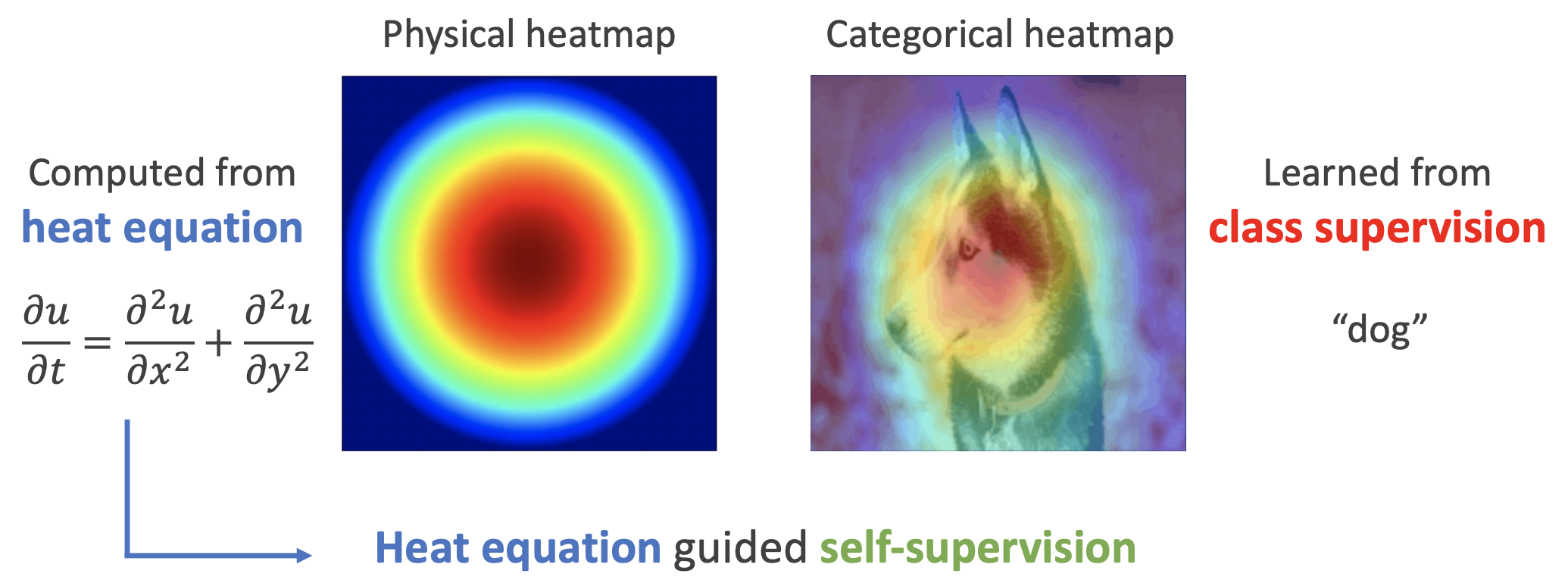 ] Heatmap of the heat equation (left) vs. heatmap of a vision model (right)
more
Specifically, the physical heat conduction equation is
\begin{equation}\frac{\partial u}{\partial t} = \frac{\partial^2 u}{\partial x^2} + \frac{\partial^2 u}{\partial y^2}\end{equation}
where $x,y$ correspond to the "width" and "height" dimensions of the image, and $u$ is the feature value at that location. Since this paper deals mainly with static images rather than video, there is no time dimension $t$, so we can simply set $\frac{\partial u}{\partial t}=0$. Since features are usually multi-dimensional vectors rather than scalars, we replace $u$ with $\boldsymbol{z}$, giving
\begin{equation}\frac{\partial^2 \boldsymbol{z}}{\partial x^2} + \frac{\partial^2 \boldsymbol{z}}{\partial y^2} = 0\label{eq:laplace}\end{equation}
This is called the "Laplace equation." It is isotropic, but images are not always isotropic, so we can introduce an additional matrix $\boldsymbol{S}$ to capture this anisotropy:
\begin{equation}\frac{\partial^2 \boldsymbol{z}}{\partial x^2} + \boldsymbol{S}\frac{\partial^2 \boldsymbol{z}}{\partial y^2} = 0\label{eq:laplace-s}\end{equation}
However, this is a second-order equation, and as we'll see later, discretizing it directly turns out to be rather cumbersome. So the authors propose converting it further into a first-order system of equations:
\begin{equation}\frac{\partial \boldsymbol{z}}{\partial x} = \boldsymbol{A}\boldsymbol{z},\quad \frac{\partial \boldsymbol{z}}{\partial y} = \boldsymbol{B}\boldsymbol{z}\label{eq:laplace-1o}\end{equation}
One can verify that as long as $\boldsymbol{S} = -\boldsymbol{A}^2(\boldsymbol{B}^2)^{-1}$, the solution of the above equation is necessarily also a solution of equation $\eqref{eq:laplace-s}$, which is why the original paper takes equation $\eqref{eq:laplace-1o}$ as its starting point.
Discrete Reconstruction
After all that, the core idea of the original paper is actually quite simple: it posits that the features obtained by passing the original image through an encoder should, as much as possible, satisfy equation $\eqref{eq:laplace-1o}$. Specifically, after passing through the encoder—prior to global pooling—the image yields a feature map of shape $w\times h\times d$, which we treat as $m\times n$ vectors of dimension $d$, or in other words, a function $\boldsymbol{z}(x, y)\in \mathbb{R}^d$, where $(x,y)$ is the position of that vector. The function $\boldsymbol{z}(x, y)$ should then satisfy equation $\eqref{eq:laplace-1o}$ as closely as possible.
How do we bring this about? Based on equation $\eqref{eq:laplace}$, we can derive the discretization scheme
\begin{equation}\begin{aligned} &\,\boldsymbol{z}(x+\Delta x, y) \approx \boldsymbol{z}(x, y) + \Delta x \boldsymbol{A}\boldsymbol{z}(x,y) = (\boldsymbol{I} + \Delta x \boldsymbol{A})\boldsymbol{z}(x,y) \\ &\,\boldsymbol{z}(x, y+\Delta y) \approx \boldsymbol{z}(x, y) + \Delta y \boldsymbol{B}\boldsymbol{z}(x,y) = (\boldsymbol{I} + \Delta y \boldsymbol{B})\boldsymbol{z}(x,y) \end{aligned}\label{eq:laplace-delta}\end{equation}
This means we can predict the features at nearby positions from the features at the current position. Based on this, the original paper proposes a self-supervised learning method called "QB-Heat":
Each time, only a small portion of the image is fed in; after passing through the encoder, we obtain the corresponding features, and use the discretized form $ > \eqref{eq:laplace-delta}$ to predict the features of the full image, which are then fed into a small decoder to reconstruct the complete image.
A schematic diagram is shown below:
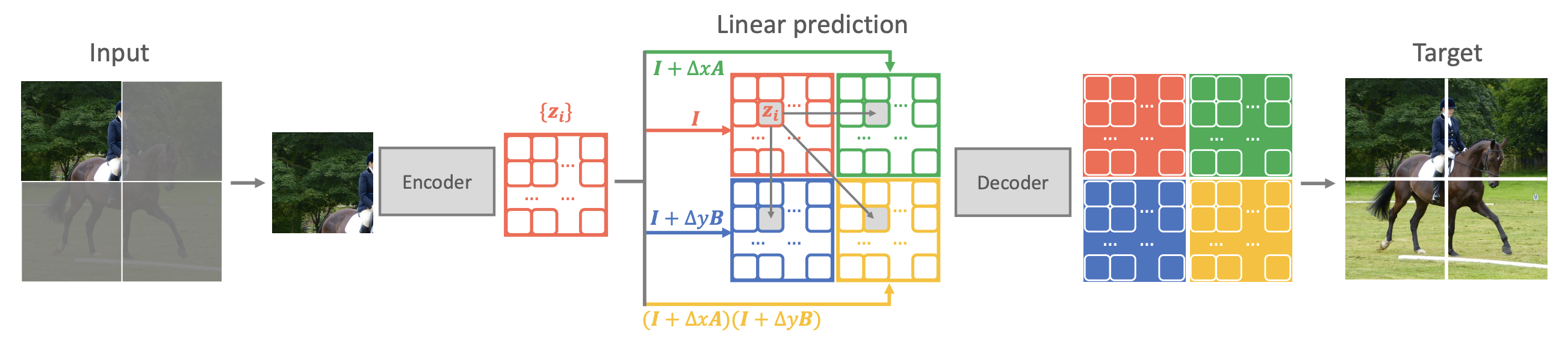 ] Schematic of the QB-Heat framework
Comparative Analysis
That covers the introduction to QB-Heat. The rest of the original paper is devoted to experimental results and some analysis that, in my view, is not all that closely related to the main point, so I'll skip over it—interested readers can just consult the original paper.
If you've read about the MAE model (see 《MLM and MAE from a Dropout Perspective: Some New Insights》]), you'll probably notice that QB-Heat has quite a lot in common with MAE—both feed a partial image into the encoder and then reconstruct the full image, and in both cases the encoder is large while the decoder is small. Aside from the masking strategy, the biggest difference between the two lies in what's fed into the decoder: QB-Heat uses the approximation $\eqref{eq:laplace-delta}$ to predict features for the rest of the image, whereas MAE simply treats the features of the remaining region as a single uniform [MASK]. It's easy to imagine that predicting via the approximation $\eqref{eq:laplace-delta}$ would naturally be more sensible than crudely filling in with [MASK], so it makes sense that QB-Heat outperforms MAE.
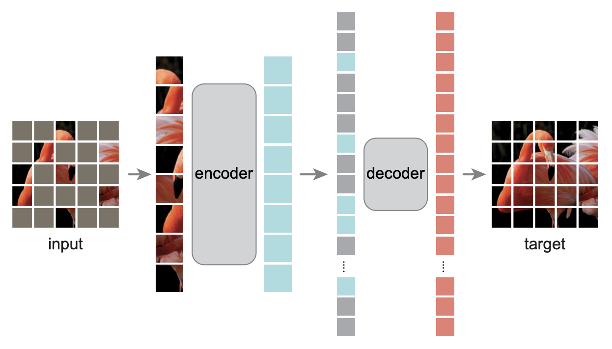 ] Schematic of the MAE model
Equation $\eqref{eq:laplace-delta}$ implies that QB-Heat can only predict the surrounding region from the center (otherwise interpolation in the middle becomes rather messy). Consequently, QB-Heat's masking strategy has to be to keep one contiguous square region and mask out everything around it, as shown in the figure below. Precisely because QB-Heat's input is a contiguous sub-image of the original, its encoder can be built with either a Transformer or a pure CNN. MAE, by contrast, randomly masks out pixels of the original image, and to achieve the effect of reducing encoder compute this way, MAE's encoder has to be a Transformer—since only a Transformer can shrink the sequence length while still preserving positional information.
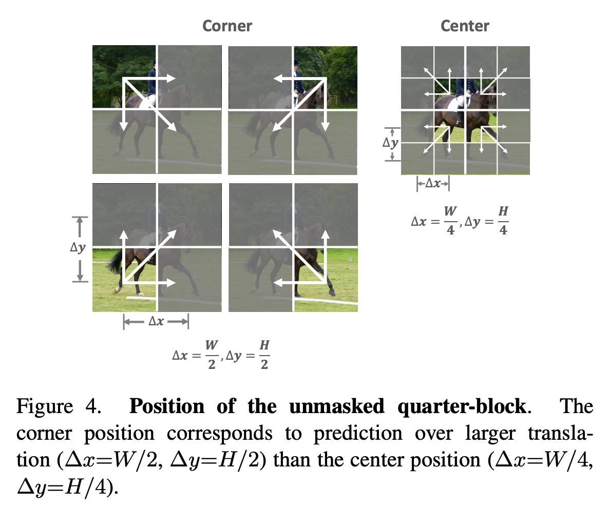 ] Schematic of QB-Heat's masking strategy
Personal Thoughts
As appealing as the physics perspective looks, it's often just a "front" (not meant pejoratively)—what matters more is seeing through the surface phenomenon to the underlying mechanism that actually makes it work.
First, one obvious "gripe" about QB-Heat is that both the title and the method are branded with the name of the heat conduction equation, yet the heat conduction equation's actual appearance in the derivation lasts, so to speak, "no more than three seconds"—giving the impression that it's dispensable. In fact, the paper's real starting point should be equation $\eqref{eq:laplace}$, the Laplace equation. Although formally the Laplace equation corresponds to the static solution of the heat conduction equation, whether viewed mathematically or physically, the two belong to different branches of study, so invoking the name "heat conduction equation" feels somewhat forced. Second, the Laplace equation actually used is not the original equation $\eqref{eq:laplace}$ or $\eqref{eq:laplace-s}$, but the simplified equation $\eqref{eq:laplace-1o}$, and in practice this corresponds to the approximation $\eqref{eq:laplace-delta}$. Setting aside the physical background and looking directly at equation $\eqref{eq:laplace-delta}$, it states the following assumption:
Neighboring feature vectors should be as similar as possible; they should differ from one another by, as much as possible, the same single linear transformation.
In plain terms, it makes an explicit prediction of feature vectors based on continuity and linearity assumptions, thereby serving as an implicit regularizer. This can't help but remind me of mixup, discussed in 《From SamplePairing to mixup: The Magical Regularization Term》], which likewise explicitly constructs data in a way that effectively injects implicit linear regularization into the model, boosting its final generalization ability.
For me, whenever I see a method from CV, I inevitably wonder whether it could be transplanted into NLP. So could QB-Heat be adapted this way? Compared with MAE, the biggest change QB-Heat makes is that the features of the remaining portion of the original image should be predicted through certain assumptions, rather than uniformly replaced with [MASK]. QB-Heat relies on continuity and linearity assumptions for CV—can the same be replicated for NLP? Language is fundamentally a time series, with only one dimension of variation, which is equivalent to asking: can we assume that the sentence vectors of adjacent sentences differ by the same linear transformation? Intuitively, natural language doesn't seem like it should exhibit that kind of nice continuity—but if we understand this purely from the angle of linear regularization, it doesn't seem infeasible either, especially since mixup works quite well on many NLP tasks too.
Additionally, if instead of keeping only a contiguous sub-range (as QB-Heat does), we randomly mask out some tokens, we could presumably also predict the feature vector at a masked position by linear interpolation between the feature vectors on either side—this too satisfies the continuity and linearity assumptions. I wonder whether this approach would work well? These are all fairly preliminary ideas that remain to be verified experimentally.
Summary
This post introduced QB-Heat, a scheme that uses the heat conduction equation to guide self-supervised learning. Its distinguishing feature relative to MAE is that it uses a simple prediction—rather than [MASK]—as the feature fed into the decoder for the remaining portion of the image.
Translated automatically with claude-sonnet-5; all equations are reproduced verbatim from the source. Copyright remains with the original author.