Generative Diffusion Models: Chapter 13 — From Universal Gravitation to Diffusion Models

生成扩散模型漫谈（十三）：从万有引力到扩散模型 苏剑林 · 2022-10-18 · Machine Learning gravity field theory generative model diffusion

For many readers, generative diffusion models are probably the first models they've encountered that manage to bring so many mathematical tools to bear on deep learning. In this series, we've already shown the deep connections between diffusion models and mathematical analysis, probability and statistics, ordinary differential equations, stochastic differential equations, and even partial differential equations. One might say that even students doing pure theoretical research in mathematical physics equations could likely find a place for their expertise within diffusion models.

In this article, we introduce another diffusion model with a profound connection to mathematical physics — an ODE-based diffusion model inspired by the "law of universal gravitation," from the paper Poisson Flow Generative Models (abbreviated PFGM). It offers an entirely new perspective on constructing ODE-based diffusion models.

Universal Gravitation

Back in middle school we all learned the law of universal gravitation, roughly stated as follows:

The mutual attractive force between two point masses is proportional to the product of their masses and inversely proportional to the square of the distance between them.

Here we'll ignore mass and constants and focus mainly on the direction of the force and its relationship with distance. Suppose the source of gravity is located at $\boldsymbol{y}$; then the gravitational force experienced by an object at $\boldsymbol{x}$ can be written as

\begin{equation}\boldsymbol{F}(\boldsymbol{x}) = -\frac{1}{4\pi}\frac{\boldsymbol{x} - \boldsymbol{y}}{\Vert \boldsymbol{x} - \boldsymbol{y}\Vert^3}\label{eq:grad-3}\end{equation}

We can set aside the factor $\frac{1}{4\pi}$ for now, since it doesn't affect the subsequent analysis. To be precise, the formula above describes the gravitational field in three-dimensional space; for $d$-dimensional space, the gravitational field takes the form

\begin{equation}\boldsymbol{F}(\boldsymbol{x}) = -\frac{1}{S_d(1)}\frac{\boldsymbol{x} - \boldsymbol{y}}{\Vert \boldsymbol{x} - \boldsymbol{y}\Vert^d}\label{eq:grad-d}\end{equation}

where $S_d(1)$ is the surface area of the $d$-dimensional unit hypersphere. This expression is actually the gradient of the Green's function of the $d$-dimensional Poisson equation — which is where the word "Poisson" in the paper's title comes from.

Following the Field Lines

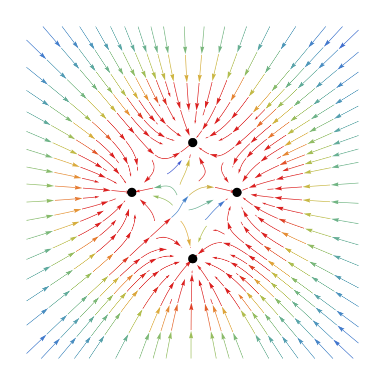
If there are multiple sources of gravity, we simply add up the gravitational fields from each source — this is the linear superposition property of gravitational fields. Below we plot the vector field of four gravity sources, with the sources marked as black dots and the colored lines representing field lines:

Gravitational field diagram

From the gravitational field plot above, we can observe an important characteristic:

With very few exceptions, most field lines originate far away and terminate at one of the gravity source points.

This suggests an intuitive, if "wild," idea:

If each gravity source represents a real sample point we want to generate, then couldn't any point far away simply follow the field lines to evolve into a real sample point?

This is the core stroke of genius in Poisson Flow Generative Models!

Equivalent Center of Mass

Of course, genius aside, there are still many details to fill in before this can become a truly usable model. For instance, we just said "any point far away" — this is meant to be the initial distribution for the diffusion model — so the question arises: how far is "far"? How should we sample this "any point"? If the sampling scheme is too complicated, it won't be of much use.

Fortunately, gravitational fields have an extremely important equivalence property:

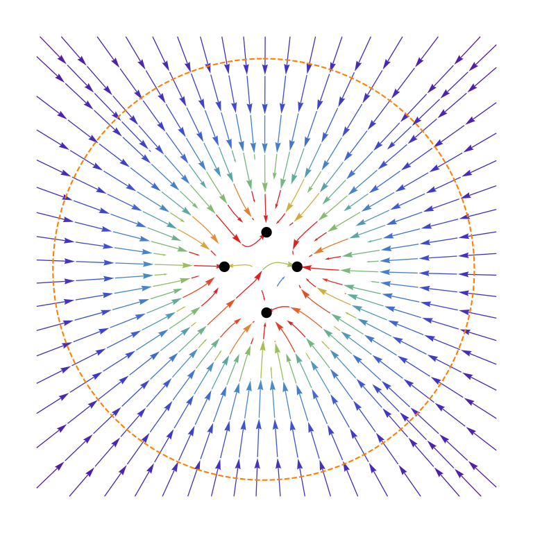
The multi-source gravitational field at infinity is equivalent to the gravitational field of a single point mass located at the center of mass, with mass equal to the sum of all source masses.

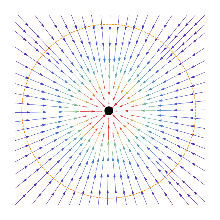
That is, when the distance is sufficiently large, we can treat the field as if it were generated by a single point mass located at the center of mass. The figure below shows both the multi-source gravitational field and its corresponding center-of-mass field; you can see that at larger distances (the orange circle region), the two fields are nearly identical.

Multi-source gravitational fieldCenter-of-mass gravitational field

What's special about the field of a single point mass? Isotropy! This means that at sufficiently large radii, the field lines can be regarded as passing uniformly through a sphere centered at the point mass. So we just need to sample uniformly on a sphere with a sufficiently large radius — this solves the problem of sampling the initial distribution. As for how large "sufficiently large" needs to be, we'll get to that later.

Mode Collapse

So is the generative model now fully constructed? Not quite. The isotropy of the gravitational field, while making the corresponding initial distribution easy to sample from, also causes gravity sources to cancel each other out, leading to a phenomenon known as "mode collapse."

Specifically, let's plot the gravitational field of sources uniformly distributed on a spherical shell; the resulting distribution looks like this:

Gravitational field with isotropically distributed sources

Notice the pattern? Outside the shell, the field is normally isotropic, but inside the shell it's completely "empty"! In other words, the gravitational fields inside the shell cancel each other out, effectively creating a vacuum zone. The author discussed this phenomenon in a popular-science blog post over a decade ago, The Uniform Force Field Inside a Spherical Shell.

This cancellation means that if we pick any sphere, the gravity sources uniformly distributed on that sphere will cancel each other out due to mutual attraction, effectively making it as if those sources didn't exist. And as we said, the way this article constructs a generative model is by having arbitrary faraway points move along field lines until they reach some gravity source. If the gravity sources cancel out, that means certain sources can never be reached — meaning certain real samples can never be generated, and the generated results will lack diversity. This is the phenomenon of "mode collapse."

Adding a Dimension

It might seem that mode collapse is unavoidable no matter what we do. This is because when constructing a generative model, we typically assume the real samples follow a continuous distribution; given this, for any chosen sphere, even if the real samples aren't uniformly distributed on that sphere, we can always pick out a "subset" that is uniformly distributed, and the gravity from that subset would cancel out — effectively making those data points vanish, triggering mode collapse.

So has this path truly reached a dead end? Not at all! This is where PFGM's second "stroke of genius" comes in: add a dimension!

We just analyzed that mode collapse is unavoidable because the assumption of a continuous distribution makes isotropy unavoidable. To avoid mode collapse, we need to find a way to eliminate the isotropy of the distribution. But the distribution of real samples is our target distribution, which we can't change — however, we can add a dimension to it. If we work in $d+1$-dimensional space, then the original $d$-dimensional distribution can be viewed as a plane within the $d+1$-dimensional space, and a plane can never be isotropic. Consider a lower-dimensional example: we know that in two-dimensional space, a "circle" is isotropic, but in three-dimensional space, it's the "sphere" that is isotropic — a circle that is isotropic in 2D is no longer isotropic when viewed from 3D.

So, suppose the real samples we want to generate originally lie in $\boldsymbol{x}\in\mathbb{R}^d$; we introduce a new dimension $t$, so that data points become $(\boldsymbol{x},t)\in\mathbb{R}^{d+1}$, and while the real samples originally followed the distribution $\boldsymbol{x}\sim \tilde{p}(\boldsymbol{x})$, we now change this to $(\boldsymbol{x},t)\sim \delta(t)\tilde{p}(\boldsymbol{x})$, where $\delta(t)$ is a Dirac distribution — this is really just placing the real samples onto the $t=0$ plane within the $d+1$-dimensional space. After this treatment, in $d+1$-dimensional space, the $t$ coordinate of real sample points is always 0, so isotropy can no longer occur (analogous to the "circle in 3D space" example above).

An Aha Moment

At first glance, adding a dimension might seem like a mere mathematical trick, but on closer reflection, we find it remarkably elegant — many details that were awkward to handle in the original $d$-dimensional space suddenly become clear in the $d+1$-dimensional space.

Based on equation $\eqref{eq:grad-d}$ and the linear superposition of gravity, we can write the gravitational field in this $d+1$-dimensional space as

\begin{equation}\begin{aligned} \boldsymbol{F}(\boldsymbol{x}, t) =&\, -\frac{1}{S_{d+1}(1)}\iint\frac{(\boldsymbol{x} - \boldsymbol{x}_0, t - t_0)}{(\Vert\boldsymbol{x} - \boldsymbol{x}_0\Vert^2 + (t - t_0)^2)^{(d+1)/2}}\delta(t_0)\tilde{p}(\boldsymbol{x}_0) d\boldsymbol{x}_0dt_0 \\ =&\, -\frac{1}{S_{d+1}(1)}\int\frac{(\boldsymbol{x} - \boldsymbol{x}_0, t)}{(\Vert\boldsymbol{x} - \boldsymbol{x}_0\Vert^2 + t^2)^{(d+1)/2}}\tilde{p}(\boldsymbol{x}_0) d\boldsymbol{x}_0 \\ \triangleq&\, (\boldsymbol{F}_{\boldsymbol{x}}, \boldsymbol{F}_t) \end{aligned}\label{eq:field}\end{equation}

where $\boldsymbol{F}_{\boldsymbol{x}}$ denotes the first $d$ components of $\boldsymbol{F}(\boldsymbol{x}, t)$, and $\boldsymbol{F}_t$ is its $d+1$-th component. We'll discuss how to learn $\boldsymbol{F}(\boldsymbol{x}, t)$ in the next section; for now assume $\boldsymbol{F}(\boldsymbol{x}, t)$ is already known, in which case the next step is to move along the field lines — that is, the trajectory of motion should always align with the direction of $\boldsymbol{F}(\boldsymbol{x}, t)$, i.e.,

\begin{equation}(d\boldsymbol{x}, dt) = (\boldsymbol{F}_{\boldsymbol{x}}, \boldsymbol{F}_t) d\tau\quad\Rightarrow\quad \frac{d\boldsymbol{x}}{dt} = \frac{\boldsymbol{F}_{\boldsymbol{x}}}{\boldsymbol{F}_t}\label{eq:ode}\end{equation}

This is the differential equation (ODE) needed for the generative process. In the earlier $d$-dimensional scheme, besides the mode collapse problem, deciding when to terminate was also a tricky detail to handle. Intuitively, one would move along the field lines until "hitting" a real sample and then stop, but judging exactly when a "hit" occurs is not straightforward. In the $d+1$-dimensional scheme, however, we know all real samples lie on the plane $t=0$, so we can naturally use $t=0$ as the termination signal.

As for the initial distribution, following the earlier discussion, it should be a "uniform distribution on a $d+1$-dimensional sphere with sufficiently large radius." But since we're now using $t=0$ as the termination signal, we might as well fix a sufficiently large value of $t=T$ (roughly on the order of $40\sim 100$), and then sample on the plane $t=T$. This turns the generative process into the motion of the differential equation $\eqref{eq:ode}$ from $t=T$ to $t=0$, making both the start and end of the generative process quite clear.

Of course, if we sample on a fixed $t=T$ plane, the distribution definitely won't be uniform. In fact, we have:

\begin{equation}p_{prior}(\boldsymbol{x}) \propto \frac{1}{(\Vert\boldsymbol{x}\Vert^2 + T^2)^{(d+1)/2}}\end{equation}

The derivation is given in the box below. Notice that the probability density depends only on the magnitude $\Vert\boldsymbol{x}\Vert$, so the sampling scheme from this distribution is to first sample the magnitude according to a specific distribution, then sample the direction uniformly, and combine the two. For sampling the magnitude, let $r=\Vert\boldsymbol{x}\Vert$; if we change variables to hyperspherical coordinates, we obtain $p_{prior}(r)\propto r^{d-1}(r^2 + T^2)^{-(d+1)/2}$, and then we can sample using the inverse cumulative distribution function method (see Variational Autoencoders (7): VAE on the Sphere (vMF-VAE)).

Derivation of the initial distribution: The field lines pass uniformly through the $d+1$-dimensional hypersphere, so the density at $(\boldsymbol{x}, T)$ is inversely proportional to $S_{d+1}(\boldsymbol{x}, T)$, i.e., $\propto \frac{1}{(\Vert\boldsymbol{x}\Vert^2 + T^2)^{d/2}}$. But now we're not on the sphere — we're on the plane $t=T$ — so we need to project the sphere onto the plane, as shown below:
Projection from sphere to the t=T plane
As shown above, when points $B$ and $D$ are sufficiently close, we have $\Delta OAB\sim \Delta BDC$, so
\begin{equation}\frac{|BC|}{|BD|} = \frac{|OB|}{|OA|} = \frac{\sqrt{\Vert\boldsymbol{x}\Vert^2 + T^2}}{T}\end{equation}
That is, an arc of unit length on the sphere, once projected onto the plane, becomes $\frac{\sqrt{\Vert\boldsymbol{x}\Vert^2 + T^2}}{T}$ times as long. Since only one dimension changes, the area element on the sphere also becomes $\frac{\sqrt{\Vert\boldsymbol{x}\Vert^2 + T^2}}{T}$ times as large after projection. Thus, since probability is inversely proportional to area, we obtain
\begin{equation}p_{prior}(\boldsymbol{x}) \propto \frac{1}{S_{d+1}(\boldsymbol{x}, T)}\times \frac{T}{\sqrt{\Vert\boldsymbol{x}\Vert^2 + T^2}}\propto \frac{1}{(\Vert\boldsymbol{x}\Vert^2 + T^2)^{(d+1)/2}}\end{equation}

Training the Field

Now that we have the initial distribution and the differential equation, all that remains is to train the vector field function $\boldsymbol{F}(\boldsymbol{x}, t)$. From the differential equation $\eqref{eq:ode}$, we can see that it depends only on the relative value of the vector field, so scaling the vector field doesn't affect the final result. Based on equation $\eqref{eq:field}$, the vector field can be written as

\begin{equation}\boldsymbol{F}(\boldsymbol{x}, t) = \mathbb{E}_{\boldsymbol{x}_0\sim \tilde{p}(\boldsymbol{x}_0)}\left[-\frac{(\boldsymbol{x} - \boldsymbol{x}_0, t)}{(\Vert\boldsymbol{x} - \boldsymbol{x}_0\Vert^2 + t^2)^{(d+1)/2}}\right]\end{equation}

Recall a result we've used several times in earlier articles, such as Generative Diffusion Models: Chapter 5 — General Framework, the SDE Perspective and Generative Diffusion Models: Chapter 7 — Optimal Diffusion Variance Estimation (Part 1):

\begin{equation}\mathbb{E}_{\boldsymbol{x}}[\boldsymbol{x}] = \mathop{\text{argmin}}_{\boldsymbol{\mu}}\mathbb{E}_{\boldsymbol{x}}\left[\Vert \boldsymbol{x} - \boldsymbol{\mu}\Vert^2\right]\end{equation}

We can introduce a function $\boldsymbol{s}_{\boldsymbol{\theta}}(\boldsymbol{x}, t)$ to learn $\boldsymbol{F}(\boldsymbol{x}, t)$, with training objective

\begin{equation}\mathbb{E}_{\boldsymbol{x}_0\sim \tilde{p}(\boldsymbol{x}_0)}\left[\left\Vert\boldsymbol{s}_{\boldsymbol{\theta}}(\boldsymbol{x}, t) + \frac{(\boldsymbol{x} - \boldsymbol{x}_0, t)}{(\Vert\boldsymbol{x} - \boldsymbol{x}_0\Vert^2 + t^2)^{(d+1)/2}}\right\Vert^2\right]\label{eq:loss}\end{equation}

However, in the objective above, $\boldsymbol{x},t$ still needs to be sampled, and its sampling method isn't clearly defined. This is actually one of the main features of PFGM: it directly defines the reverse process (the generative process) without needing to define a forward process — this sampling step effectively plays the role of the forward process. To this end, the original paper constructs samples of $\boldsymbol{x},t$ by perturbing each real sample as follows:

\begin{equation}\boldsymbol{x} = \boldsymbol{x}_0 + \Vert \boldsymbol{\varepsilon}_{\boldsymbol{x}}\Vert (1+\tau)^m \boldsymbol{u},\quad t = |\varepsilon_t| (1+\tau)^m\end{equation}

where $(\boldsymbol{\varepsilon}_{\boldsymbol{x}},\varepsilon_t)\sim\mathcal{N}(\boldsymbol{0}, \sigma^2\boldsymbol{I}_{(d+1)\times(d+1)})$, $m\sim U[0,M]$, $\boldsymbol{u}$ is a unit vector uniformly distributed on the $d$-dimensional unit sphere, and $\tau,\sigma,M$ are all constants. There's considerable subjectivity in this design; readers can appreciate and interpret it for themselves — we won't dwell on it further here. For further discussion, see here.

Finally, the training objective in the original paper differs slightly from equation $\eqref{eq:loss}$ in this article; it's roughly equivalent to

\begin{equation}\left\Vert\boldsymbol{s}_{\boldsymbol{\theta}}(\boldsymbol{x}, t) + \text{Normalize}\left(\mathbb{E}_{\boldsymbol{x}_0\sim \tilde{p}(\boldsymbol{x}_0)}\left[\frac{(\boldsymbol{x} - \boldsymbol{x}_0, t)}{(\Vert\boldsymbol{x} - \boldsymbol{x}_0\Vert^2 + t^2)^{(d+1)/2}}\right]\right)\right\Vert^2\end{equation}

In actual training, since only a finite number of $\boldsymbol{x}_0$ samples can be drawn to estimate the expectation inside the brackets, this objective is actually a biased estimator. Of course, biased doesn't necessarily mean worse than unbiased. Exactly why the original paper uses a biased estimator isn't entirely clear to me at the moment — my guess is that the biased estimator, by normalizing the vectors, might make the training process more stable. But because the biased estimate involves normalization, it requires a larger batch size to be accurate, which raises the bar for experimental cost.

Experimental Results

It's fair to say that PFGM is a thoroughly new framework — it no longer relies on the Gaussian assumption as before, and yields a model with genuinely novel content. That said, we shouldn't pursue "novelty for novelty's sake." If a new framework doesn't produce more convincing results, then the novelty is meaningless.

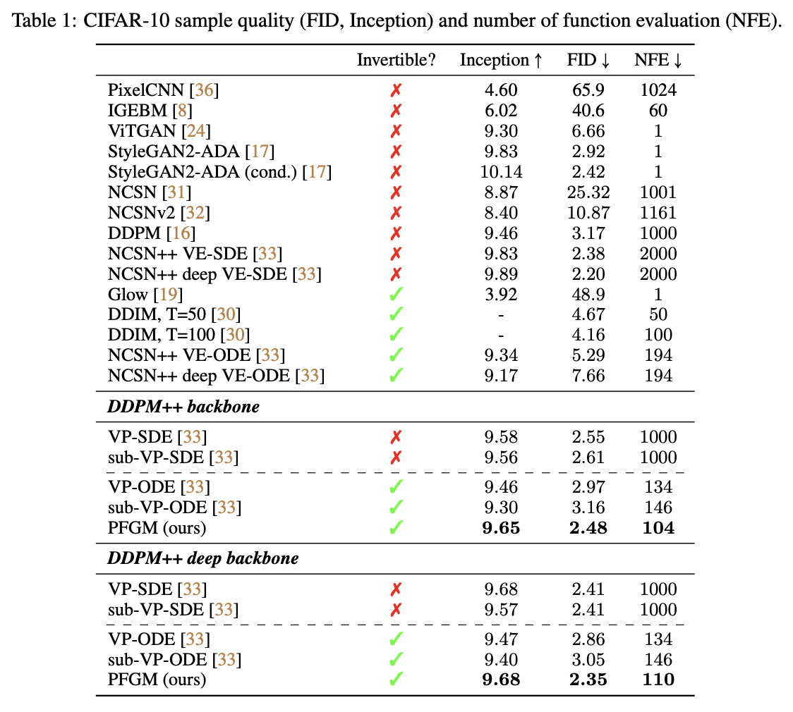
Fortunately, the experimental results in the original paper do confirm the value of PFGM — for instance, achieving better evaluation metrics, faster generation speed, and greater robustness to hyperparameters (including model architecture), among other things. We won't go through all of these here; interested readers should consult the original paper. Having looked at the paper, which was accepted at NeurIPS 2022, I have to say it's truly a top-conference paper that lives up to its reputation!

Official GitHub: https://github.com/Newbeeer/Poisson_flow

PFGM experimental results (partial)

Summary

This article introduced an ODE-based diffusion model inspired by the "law of universal gravitation," which breaks free from the reliance on Gaussian assumptions found in many previous diffusion models. It represents an entirely new framework for constructing ODE-based diffusion models grounded in field theory, and the whole model is highly thought-provoking and well worth studying carefully.