MLM and MAE Through the Lens of Dropout: Some New Insights

Dropout视角下的MLM和MAE：一些新的启发 苏剑林 · 2021-11-29 · Machine Learning model probability analysis optimization

Everyone knows that BERT's MLM (Masked Language Model) task suffers from an inconsistency between pretraining and fine-tuning — namely, [MASK] tokens appear during pretraining but not during downstream fine-tuning. This is a frequently criticized issue, and many works consider it an important factor hurting BERT's fine-tuning performance, leading to a number of targeted improvements such as XL-NET, ELECTRA, MacBERT, and others. In this post, we'll analyze this inconsistency in MLM from the perspective of Dropout, and propose a simple operation to correct it.

The same analysis can also be applied to the recently popular MAE (Masked Autoencoder) model proposed by Kaiming He. It turns out that MAE indeed has better consistency than MLM, and from this we can derive a regularization technique that may speed up training.

Dropout

Let's first review Dropout. Mathematically speaking, Dropout introduces random noise into the model via a Bernoulli distribution, so let's briefly review the Bernoulli distribution too.more

The Bernoulli Distribution

The Bernoulli distribution is arguably the simplest probability distribution — it's a two-valued distribution over $\{0,1\}$, where $\varepsilon$ takes the value 1 with probability $p$ and 0 with probability $1-p$, denoted as

\begin{equation}\varepsilon\sim \text{Bernoulli}(p)\end{equation}

An interesting property of the Bernoulli distribution is that all of its moments equal $p$, i.e.

\begin{equation}\mathbb{E}_{\varepsilon}[\varepsilon^n] = p\times 1^n + (1-p)\times 0^n = p\end{equation}

So we know its mean is $p$, and its variance is

\begin{equation}\mathbb{V}ar_{\varepsilon}[\varepsilon] = \mathbb{E}_{\varepsilon}[\varepsilon^2] - \mathbb{E}_{\varepsilon}[\varepsilon]^2 = p(1-p)\end{equation}

Training and Inference

During training, Dropout zeroes out certain values with probability $1-p$, while the remaining values are divided by $p$. So Dropout effectively introduces a random variable $\varepsilon\sim \text{Bernoulli}(p)$, turning the model from $f(x)$ into $f(x\varepsilon/p)$. Here $\varepsilon$ may have multiple components corresponding to multiple independent Bernoulli distributions, but in most cases the result is not fundamentally different from treating $\varepsilon$ as a scalar, so we only need to work out the derivation for the case where $\varepsilon$ is a scalar.

In Dropout Twice Again! This Time It Achieves SOTA on a Supervised Task] we proved that if the loss function is MSE, then the optimal prediction model after training should be

\begin{equation}\mathbb{E}_{\varepsilon}[f(x\varepsilon/p)]\end{equation}

This means that, ideally, we should predict multiple times without turning off Dropout, and then average the predictions as the final result — i.e. perform "model averaging." But this is clearly computationally expensive, so in practice we rarely do this; instead, we simply turn off Dropout, i.e. set $\varepsilon/p$ to 1. And we know that

\begin{equation}f(x)=f(x\,\mathbb{E}_{\varepsilon}[\varepsilon]/p)\end{equation}

So turning off Dropout is in fact a form of "weight averaging" (treating $\varepsilon$ as the model's random weight). In other words, the theoretically optimal solution is "model averaging," but for computational reasons we typically approximate it with "weight averaging," which can be viewed as a first-order approximation of "model averaging."

The MLM Model

In this section, we treat the MLM model as a special case of Dropout, which lets us clearly describe the inconsistency between pretraining and fine-tuning, and derive a simple correction strategy that can better alleviate this inconsistency.

The Dropout Perspective

For simplicity, let's first analyze a simplified version of MLM: suppose that during pretraining, each token keeps its original value with probability $p$, and is replaced with [MASK] with probability $1-p$. Let the embedding of the $i$-th token be denoted $x_i$, and the embedding of [MASK] be $m$. We can then similarly introduce a random variable $\varepsilon\sim \text{Bernoulli}(p)$, and write the MLM model as

\begin{equation}f(\cdots,x_i,\cdots)\quad\rightarrow\quad f(\cdots,x_i \varepsilon + m(1-\varepsilon),\cdots)\end{equation}

In this way, MLM is essentially the same as Dropout — both introduce random perturbations into the model via a Bernoulli distribution. Now, following the standard usage of Dropout, its prediction model should use "weight averaging," i.e.

\begin{equation}f(\cdots,\mathbb{E}_{\varepsilon}[x_i \varepsilon + m(1-\varepsilon)],\cdots) = f(\cdots,x_i p + m (1-p),\cdots)\end{equation}

Here the inconsistency of MLM during fine-tuning becomes apparent: if we view pretrained MLM as a special form of Dropout, then fine-tuning corresponds to "turning off Dropout." Following standard practice, we should then replace each token's embedding with $x_i p + m (1-p)$ — but in fact we don't; instead, we keep the original $x_i$.

Correcting the Embeddings

Under BERT's default settings, during MLM training, 15% of the tokens are selected for MLM prediction, and among those 15% of tokens, 80% are replaced with [MASK], 10% are kept unchanged, and the remaining 10% are randomly replaced with a random token. Based on the above analysis, after MLM pretraining is complete, we should adjust the embeddings as follows:

\begin{equation}\text{Embedding[i]} \leftarrow 0.85\times \text{Embedding[i]} + 0.15\times\left(\begin{array}{l}0.8\times \text{Embedding[m]} \,+\\ 0.1 \times \text{Embedding[i]} \,+ \\ 0.1\times \text{Avg[Embedding]}\end{array}\right) \end{equation}

where $\text{Embedding[m]}$ is the embedding of [MASK], and $\text{Avg[Embedding]}$ is the average embedding over all tokens. In bert4keras, reference code looks like this:

embeddings = model.get_weights()[0]  # 一般第一个权重就是Token Embedding
v1 = embeddings[tokenizer._token_mask_id][None]  # [MASK]的Embedding
v2 = embeddings.mean(0)[None]  # 平均Embedding
embeddings = 0.85 * embeddings + 0.15 * (0.8 * v1 + 0.1 * embeddings + 0.1 * v2)  # 加权平均
K.set_value(model.weights[0], embeddings)  # 重新赋值

So, does this modification actually improve things as we'd expect? The author compared the experimental results of BERT and RoBERTa before and after this modification on CLUE (the baseline code is from bert4keras in Hand, I Have the CLUE Benchmark Baseline]), and the conclusion was "no significant change."

At this point, readers might feel a bit let down — was all that discussion above for nothing? The author believes that the above operation does indeed help alleviate the pretraining-fine-tuning inconsistency (otherwise, wouldn't we be contradicting Dropout itself?); as for why the modified version shows no improvement, it suggests that this inconsistency issue isn't as serious as we might have imagined — at least not for CLUE-style tasks. A similar result appears in MacBERT, which corrects this inconsistency during pretraining by replacing [MASK] with synonyms; the author also tested MacBERT with the same baseline code, and the results showed no significant difference from RoBERTa either. So perhaps it's only for certain specific tasks, or with larger masking ratios, that the necessity of correcting this inconsistency would become apparent.

The MAE Model

Many readers have probably already heard of the recently proposed MAE (Masked Autoencoder) model] by Kaiming He, which introduces the MLM task into image pretraining in a simple and efficient way, achieving effective improvements. In this section, we'll see that MAE can likewise be understood as a special form of Dropout, from which we can derive a new method for preventing overfitting.

The Dropout Perspective

As shown in the figure below, MAE splits the model into an encoder and a decoder, with a "deep encoder, shallow decoder" design. It places [MASK] tokens only in the decoder, while the encoder does not process [MASK] tokens at all. This means the sequence the encoder needs to process becomes much shorter. Crucially, MAE uses a masking ratio of 75%, meaning the encoder's sequence length is only 1/4 of the usual length. Combined with the "deep encoder, shallow decoder" design, the overall pretraining speed increases by more than 3x!

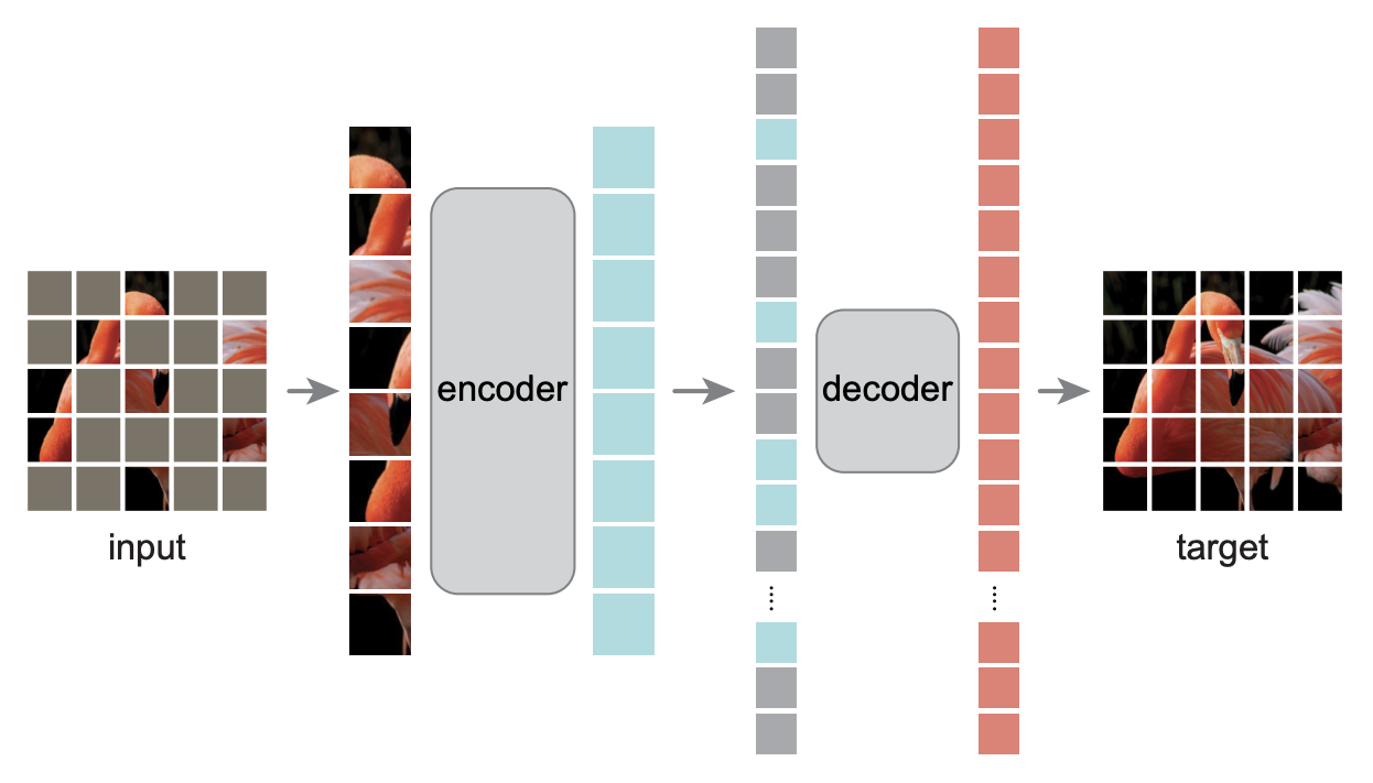Diagram of the MAE model

We can also implement the MAE model from another angle: removing [MASK] tokens from the encoder is equivalent to saying that the remaining tokens do not interact with the masked-out tokens. For a Transformer model, token interactions come from self-attention, so we could equally well keep the original input sequence intact, but mask out the corresponding columns in the attention matrix. As shown in the figure, suppose the $i$-th token is masked out — this is effectively the same as forcing all elements in the $i$-th column of the attention matrix to zero:

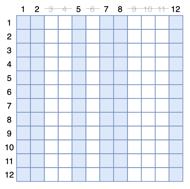Equivalent Attention-Dropout view of MAE

Of course, from a practical standpoint, this approach is purely a waste of compute, but it helps us obtain an interesting theoretical result. Suppose we have $n$ input tokens, with the original (post-softmax) attention matrix $A$. Define $M_i$ as a $n\times n$ matrix whose $i$-th column is 0 and all other entries are 1, and then define a random matrix $\tilde{M}_i$, which is the all-ones matrix with probability $p$, and equals $M_i$ with probability $1-p$. Then the MAE model can be written as

\begin{equation}f(\cdots,A,\cdots)\quad\rightarrow\quad f(\cdots,\text{Norm}(A\otimes \tilde{M}_1\otimes \tilde{M}_2\otimes \cdots\otimes \tilde{M}_n),\cdots)\end{equation}

Here $\text{Norm}$ denotes row-wise renormalization of the matrix; $\otimes$ denotes element-wise multiplication; and when there are multiple attention layers, all attention layers share the same $\tilde{M}_1,\tilde{M}_2,\cdots,\tilde{M}_n$.

In this way, we've converted MAE into a special form of Attention Dropout. Following the same "turn off Dropout" approach for the fine-tuning phase, we know the corresponding model should be

\begin{equation}\begin{aligned} &\,f(\cdots,\text{Norm}(A\otimes \mathbb{E}[\tilde{M}_1\otimes \tilde{M}_2\otimes \cdots\otimes \tilde{M}_n]),\cdots)\\ =&\,f(\cdots,\text{Norm}(A\otimes \mathbb{E}[\tilde{M}_1]\otimes \mathbb{E}[\tilde{M}_2]\otimes \cdots\otimes \mathbb{E}[\tilde{M}_n]),\cdots)\\ =&\,f(\cdots,\text{Norm}(Ap),\cdots)\\ =&\,f(\cdots,A,\cdots) \end{aligned}\end{equation}

Here the second equality holds because $\mathbb{E}[\tilde{M}_i]$ is a matrix whose $i$-th column is $p$ and whose remaining entries are 1, so $\mathbb{E}[\tilde{M}_1]\otimes \mathbb{E}[\tilde{M}_2]\otimes \cdots\otimes \mathbb{E}[\tilde{M}_n]$ is in fact an all-$p$ matrix; multiplying by it is equivalent to multiplying $A$ — that is, $A$ — directly by the constant $p$. The third equality holds because multiplying every element by the same constant doesn't affect the renormalization result.

From this result we see that for MAE, "turning off Dropout" gives a model consistent with the original one. This shows that, compared to the original MLM model, MAE offers not just a speedup but also better consistency between pretraining and fine-tuning.

Preventing Overfitting

Turning this around: since MAE can also be viewed as a form of Dropout, and Dropout helps prevent overfitting, could we use MAE's approach as a regularization technique to prevent overfitting? As shown in the figure below, during training we could randomly drop some tokens while keeping the original positions of the remaining tokens — let's call this "DropToken":

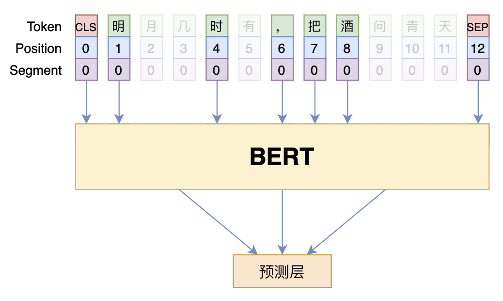DropToken diagram

The reason for thinking along these lines is that although standard Dropout is often intuitively understood as sampling a sub-network to train, this is purely an intuitive picture — in reality, adding Dropout also slows down training. DropToken, on the other hand, explicitly shortens the sequence length, so it can actually speed up training. If it works, it would be a genuinely practical trick. In addition, some readers may have already tried data augmentation by deleting certain words; the difference from DropToken is that while DropToken also removes some tokens, it retains the original positions of the remaining tokens — an implementation that relies on the Transformer architecture itself.

Here are a few experimental comparisons on CLUE, with BERT base as the baseline model; the subscript numbers indicate the drop ratio. The final results were mixed — aside from a clear improvement on IFLYTEK, the rest is somewhat down to luck (as is often the case with overfitting-prevention techniques). The optimal drop ratio seems to be between 0.1 and 0.15:

$$\begin{array}{c} \text{CLUE classification comparison (val set)} \\ {\begin{array}{c|ccccccc} \hline & \text{IFLYTEK} & \text{TNEWS} & \text{AFQMC} & \text{OCNLI} & \text{WSC} & \text{CSL} \\ \hline \text{BERT}_{\text{0.00}} & 60.06 & 56.80 & 72.41 & 73.93 & 78.62 & 83.93 \\ \text{BERT}_{\text{0.10}} & 60.56 & 57.00 & 72.61 & 73.76 & 77.30 & 83.33\\ \text{BERT}_{\text{0.15}} & 60.10 & 56.68 & 72.50 & 74.54 & 77.30 & 83.30\\ \text{BERT}_{\text{0.25}} & 61.29 & 56.88 & 72.34 & 73.09 & 73.68 & 83.37\\ \text{BERT}_{\text{0.50}} & 61.45 & 57.02 & 69.76 & 70.68 & 69.41 & 82.56\\ \hline \end{array}} \end{array}$$

Summary

In this post, we examined the MLM and MAE models from the perspective of Dropout, showing that both can be viewed as special cases of Dropout. From this perspective, we derived a technique for correcting the inconsistency in MLM, as well as an MAE-inspired technique for preventing overfitting.