Integrated Gradients: A Novel Method for Neural Network Visualization

积分梯度：一种新颖的神经网络可视化方法 苏剑林 · 2020-06-28 · Machine Learning integral gradient visualization

This post introduces a visualization method for neural networks called Integrated Gradients. It was first proposed in the paper Gradients of Counterfactuals, and later reintroduced in Axiomatic Attribution for Deep Networks, both written by the same authors and largely overlapping in content. The latter is somewhat more accessible, so if you want to read the original papers, I'd recommend starting with that one. Of course, this is work from around 2016–2017, so "novel" here refers to the cleverness of the idea rather than its recency.

Roughly speaking, visualization means: given an input $x$ and a model $F(x)$, we want to figure out which components of $x$ have the greatest influence on the model's decision — that is, to rank the importance of the components of $x$. In technical jargon, this is called "attribution." A naive approach is to directly use the gradient $\nabla_x F(x)$ as an importance measure for the components of $x$, and Integrated Gradients is an improvement on this idea. However, I feel that many articles introducing Integrated Gradients (including the original papers) are overly "mechanical" (formalistic) and fail to bring out the essential reason why Integrated Gradients works better than the naive gradient. This post tries to explain Integrated Gradients from my own angle. more

Naive Gradients

Let's start by looking at gradient-based methods, which are actually grounded in Taylor expansion:

\begin{equation}F(x+\Delta x) - F(x) \approx \langle\nabla_x F(x), \Delta x\rangle=\sum_i [\nabla_x F(x)]_i \Delta x_i\label{eq:g}\end{equation}

We know that $\nabla_x F(x)$ is a vector of the same size as $x$, where $[\nabla_x F(x)]_i$ denotes its $i$-th component. Then, for a fixed-size $\Delta x_i$, the larger the absolute value of $[\nabla_x F(x)]_i$, the larger the resulting change in $F(x+\Delta x)$ relative to $F(x)$. In other words:

$[\nabla_x F(x)]_i$ measures the model's sensitivity to the $i$-th component of the input, so we use $|[\nabla_x F(x)]_i|$ as the importance measure for the $i$-th component.

This idea is fairly simple and direct, and it's described in the papers How to Explain Individual Classification Decisions and Deep Inside Convolutional Networks: Visualising Image Classification Models and Saliency Maps. In many cases it does successfully explain predictions, but it also has an obvious drawback. Many articles have pointed out the issue of saturation regions — once you enter a saturation region (a typical example being the negative half of $\text{relu}$), the gradient becomes zero, and no useful information can be extracted.

From a practical standpoint, this explanation is reasonable, but I don't think it's deep enough. As we saw in an earlier post "A Brief Discussion of Adversarial Training: Meaning, Methods, and Reflections (with Keras Implementation)", the objective of adversarial training can be understood as pushing $\Vert\nabla_x F(x)\Vert^2 \to 0$ toward some target. This tells us that gradients can be "manipulated" — even without affecting the model's prediction accuracy, we can drive the gradient arbitrarily close to zero. So, coming back to the theme of this post: $[\nabla_x F(x)]_i$ does indeed measure the model's sensitivity to the $i$-th component of the input, but sensitivity alone is not a good measure of importance.

Integrated Gradients

Given the shortcomings of directly using the gradient described above, a number of improvements have been proposed, such as LRP and DeepLift. That said, I personally find the improvement offered by Integrated Gradients to be the cleanest and most elegant.

Reference Background

First, we need to reframe the original problem: our goal is to find the important components, but this importance shouldn't be absolute — it should be relative. For example, suppose we want to identify currently trending buzzwords. We can't just rank words by raw frequency, since that would simply surface stopwords like "的" and "了." Instead, we should prepare a "reference" frequency table computed from a balanced corpus, and then compare the differences in frequency rather than absolute values. This suggests that, in order to measure the importance of each component of $x$, we also need a "reference background" $\bar{x}$.

Of course, in many scenarios we can simply take $\bar{x}=0$, but this isn't necessarily optimal. For instance, we could instead choose $\bar{x}$ to be the mean of all training samples. We'd expect $F(\bar{x})$ to yield a fairly trivial prediction — for a classification model, say, the prediction at $\bar{x}$ should assign roughly equal probability to every class. So we turn to consider $F(\bar{x})-F(x)$, which we can think of as the "cost" of moving from $x$ to $\bar{x}$.

If we again use the approximate expansion $\eqref{eq:g}$, we obtain

\begin{equation}F(\bar{x})-F(x) \approx \sum_i [\nabla_x F(x)]_i [\bar{x} - x]_i\label{eq:g2}\end{equation}

This gives us a new way of interpreting the expression above:

The total cost of moving from $x$ to $\bar{x}$ is $F(\bar{x})-F(x)$, which is the sum of the costs contributed by each component, and the cost contributed by each component is approximately $[\nabla_x F(x)]_i [\bar{x} - x]_i$. So we can use $|[\nabla_x F(x)]_i [\bar{x} - x]_i|$ as the importance measure for the $i$-th component.

Now, whether we use $[\nabla_x F(x)]_i$ or $|[\nabla_x F(x)]_i [\bar{x} - x]_i|$, they share the same mathematical flaw (vanishing gradients), but the underlying explanations differ. As noted earlier, the flaw in $[\nabla_x F(x)]_i$ comes from the fact that "sensitivity is not a good enough measure of importance." But following the reasoning of this section, the flaw in $|[\nabla_x F(x)]_i [\bar{x} - x]_i|$ arises only because "equation $\eqref{eq:g2}$ is merely an approximation" — the logical reasoning itself is otherwise sound.

An Exact Integral Identity

Often a new way of framing a problem gives us fresh insight, which in turn inspires improvements. As just discussed, the issue boils down to "$|[\nabla_x F(x)]_i [\bar{x} - x]_i|$ isn't good enough because equation $\eqref{eq:g2}$ isn't precise enough." So if we could find an exact analogous expression, we would solve the problem. Integrated Gradients does exactly that: let $\gamma(\alpha),\alpha\in[0,1]$ denote a parametric curve connecting $x$ and $\bar{x}$, where $\gamma(0)=x, \gamma(1)=\bar{x}$. Then we have the identity

\begin{equation}\begin{aligned} F(\bar{x})-F(x) =&\, F(\gamma(1))-F(\gamma(0))\\ =& \int_0^1 \frac{dF(\gamma(\alpha))}{d\alpha}d\alpha\\ =& \int_0^1 \left\langle\nabla_{\gamma} F(\gamma(\alpha)), \gamma'(\alpha)\right\rangle d\alpha\\ =& \sum_i \int_0^1 \left[\nabla_{\gamma} F(\gamma(\alpha))\right]_i \left[\gamma'(\alpha)\right]_i d\alpha \end{aligned}\label{eq:g3}\end{equation}

Notice that equation $\eqref{eq:g3}$ has the same form as $\eqref{eq:g2}$, except that $[\nabla_x F(x)]_i [\bar{x} - x]_i$ has been replaced with $\int_0^1 \left[\nabla_{\gamma} F(\gamma(\alpha))\right]_i \left[\gamma'(\alpha)\right]_i d\alpha$. But equation $\eqref{eq:g3}$ is an exact integral identity, so Integrated Gradients proposes using

\begin{equation}\left|\int_0^1 \left[\nabla_{\gamma} F(\gamma(\alpha))\right]_i \left[\gamma'(\alpha)\right]_i d\alpha\right|\label{eq:ig-1}\end{equation}

as the importance measure for the $i$-th component. The simplest choice is to take $\gamma(\alpha)$ to be the straight line between the two points, i.e.,

\begin{equation}\gamma(\alpha) = (1 - \alpha) x + \alpha \bar{x}\end{equation}

in which case Integrated Gradients takes the concrete form

\begin{equation}\left|\left[\int_0^1 \nabla_{\gamma} F(\gamma(\alpha))\big|_{\gamma(\alpha) = (1 - \alpha) x + \alpha \bar{x}}d\alpha\right]_i \left[\bar{x}-x\right]_i\right|\label{eq:ig-2}\end{equation}

So, compared with $|[\nabla_x F(x)]_i [\bar{x} - x]_i|$, the difference is that we replace $\nabla_x F(x)$ with the integral of the gradient $\int_0^1 \nabla_{\gamma} F(\gamma(\alpha))\big|_{\gamma(\alpha) = (1 - \alpha) x + \alpha \bar{x}}d\alpha$ — that is, the average gradient over every point on the straight line from $x$ to $\bar{x}$. Intuitively, since we now account for the gradient at every point along the entire path, we're no longer limited by the gradient vanishing at any single point.

If you've read the two original Integrated Gradients papers, you'll notice their presentation runs in the opposite order: they mysteriously introduce equation $\eqref{eq:ig-2}$ first, then prove that it satisfies two seemingly arbitrary properties (sensitivity and implementation invariance), and only afterward show that it satisfies equation $\eqref{eq:g3}$. In short, the reader is led on a long detour without ever clearly stating the essential reason why it's a better importance measure — namely, that both approaches are based on decomposing $F(\bar{x})-F(x)$, and equation $\eqref{eq:g3}$ is simply more precise than equation $\eqref{eq:g2}$.

Discrete Approximation

Finally, how do we actually compute this integral quantity? Deep learning frameworks don't have a built-in integration operation. Fortunately, it's simple: following the "approximate-then-take-the-limit" definition of the integral, we can just use a discrete approximation directly. Taking equation $\eqref{eq:ig-2}$ as an example, it can be approximated as:

\begin{equation}\left|\left[\frac{1}{n}\sum_{k=1}^n\Big(\nabla_{\gamma} F(\gamma(\alpha))\big|_{\gamma(\alpha) = (1 - \alpha) x + \alpha \bar{x}, \alpha=k/n}\Big)\right]_i \left[\bar{x}-x\right]_i\right|\end{equation}

So, once again, the essence of the method is "the average gradient over every point on the line from $x$ to $\bar{x}$," which performs better than the gradient at a single point.

Experimental Results

Having covered the theory, let's look at some experimental results.

Original Results

Original paper's implementation: https://github.com/ankurtaly/Integrated-Gradients

Below are some illustrations from the original paper:

Comparison of gradients and Integrated Gradients in the original paper (a CV task; note how Integrated Gradients highlights key features more precisely)

Comparison of gradients and Integrated Gradients in the original paper (an NLP task; red indicates positive correlation, blue indicates negative correlation, gray indicates no correlation)

My Own Implementation

Although Keras's official website already provides a reference implementation (see here), the code is quite long and tedious to read, so I implemented my own version in Keras based on my understanding, and applied it to an NLP task. The code can be found at "task_sentiment_integrated_gradients.py". The current code is just a simple demo, and readers are welcome to build more powerful versions on top of it.

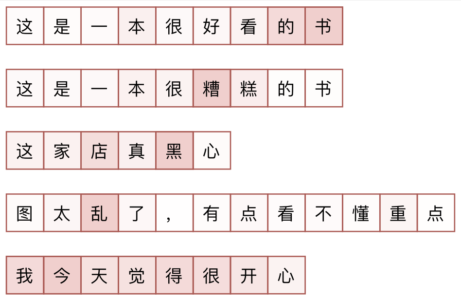My experimental results applying Integrated Gradients to Chinese sentiment classification (the redder the token, the more important it is)

The figure above shows results for a few samples (the model correctly predicted the sentiment label for all of them), from which we can infer something about how the original model performs sentiment classification. As shown, for negative samples, Integrated Gradients quite reasonably locates the negative words in the sentence, whereas for positive samples — even ones with the same grammatical structure as the negative ones — it fails to locate any positive words. This suggests that the model's approach to sentiment classification may essentially be "negativity detection": it primarily detects negative sentiment, and treats the absence of detected negativity as a positive prediction. This is likely a consequence of never having been trained on "neutral" examples.

Closing Remarks

This post introduced a neural network visualization method called "Integrated Gradients," which can, to some extent, better characterize the importance of each component of the input. By integrating the gradient along a path, Integrated Gradients constructs an exact identity that compensates for the imprecision of the Taylor expansion, thereby achieving better visualization results than directly using the gradient.