Generative Diffusion Models Explained (X): Unified Diffusion Models (Theory)

生成扩散模型漫谈（十）：统一扩散模型（理论篇） 苏剑林 · 2022-09-14 · Machine Learning unification generative model DDPM diffusion

Longtime readers may notice that, compared with the previous update pace, this post has been rather "slow to arrive," because there was simply too much to think through.

Over the previous nine posts, we've given a fairly comprehensive introduction to generative diffusion models. Although there's already a lot of theoretical content, we can see that the diffusion models discussed so far all deal with continuous objects, and all build the forward process based on Gaussian noise. This "overthought" post hopes to construct a unified diffusion model framework (Unified Diffusion Model, UDM) that breaks through these limitations:

1. Not restricted to any particular type of object (can be continuous $\boldsymbol{x}$ or discrete $\boldsymbol{x}$);
2. Not restricted to any particular forward process (the forward process can be built using noising, blurring, masking, deletion, or various other transformations);
3. Not restricted to any particular type of time (can be discrete $t$ or continuous $t$);
4. Encompasses existing results (should be able to recover previous results such as DDPM, DDIM, SDE, ODE, etc.).

Isn't this a bit too "wishful thinking"? Is there really such an ideal framework? This post is an attempt to find out. more

The Forward Process

From the series of posts so far, we know that building a diffusion model involves three components: the "forward process," the "reverse process," and the "training objective." In this section we analyze the forward process.

In the original DDPM, we described the forward process via $p(\boldsymbol{x}_t|\boldsymbol{x}_{t-1})$; later, as works like DDIM were published, we gradually realized that the training objective and the generative process of diffusion models don't actually have a direct connection to $p(\boldsymbol{x}_t|\boldsymbol{x}_{t-1})$, but instead are more directly connected to $p(\boldsymbol{x}_t|\boldsymbol{x}_0)$, and deriving $p(\boldsymbol{x}_t|\boldsymbol{x}_0)$ from $p(\boldsymbol{x}_t|\boldsymbol{x}_{t-1})$ is often quite difficult. Hence, a more practical approach is to start directly from $p(\boldsymbol{x}_t|\boldsymbol{x}_0)$, that is, to treat $p(\boldsymbol{x}_t|\boldsymbol{x}_0)$ as the forward process.

The most direct role of $p(\boldsymbol{x}_t|\boldsymbol{x}_0)$ is to construct training data for the diffusion model, so the most basic requirement for $p(\boldsymbol{x}_t|\boldsymbol{x}_0)$ is that it be easy to sample from. To this end, we can use the reparameterization

\begin{equation}\boldsymbol{x}_t = \boldsymbol{\mathcal{F}}_t(\boldsymbol{x}_0,\boldsymbol{\varepsilon})\label{eq:re-param}\end{equation}

where $\boldsymbol{\mathcal{F}}$ is a deterministic function of $t,\boldsymbol{x}_0,\boldsymbol{\varepsilon}$, and $\boldsymbol{\varepsilon}$ is a random variable sampled from some standard distribution $q(\boldsymbol{\varepsilon})$; a common choice is the standard normal distribution, though other distributions are typically feasible too. As one can imagine, this form encompasses a sufficiently rich family of transformations from $\boldsymbol{x}_0$ to $\boldsymbol{x}_t$, and it places no constraint on the data types of $\boldsymbol{x}_0$ and $\boldsymbol{x}_t$. In general, the only restriction is that the smaller $t$ is, the more completely $\boldsymbol{\mathcal{F}}_t(\boldsymbol{x}_0,\boldsymbol{\varepsilon})$ preserves the information of $\boldsymbol{x}_0$ — in other words, the easier it is to reconstruct $\boldsymbol{x}_0$ from $\boldsymbol{\mathcal{F}}_t(\boldsymbol{x}_0,\boldsymbol{\varepsilon})$ — whereas the larger $t$ is, the harder reconstruction becomes, until at some upper bound $T$ the information about $\boldsymbol{x}_0$ contained in $\boldsymbol{\mathcal{F}}_T(\boldsymbol{x}_0,\boldsymbol{\varepsilon})$ has essentially vanished, and reconstruction becomes nearly impossible.

The Reverse Process

The reverse process of a diffusion model gradually generates realistic data through multi-step iteration, and the key to this is the probability distribution $p(\boldsymbol{x}_{t-1}|\boldsymbol{x}_t)$. In general, we have

\begin{equation}p(\boldsymbol{x}_{t-1}|\boldsymbol{x}_t) = \int p(\boldsymbol{x}_{t-1}|\boldsymbol{x}_t, \boldsymbol{x}_0) p(\boldsymbol{x}_0|\boldsymbol{x}_t) d\boldsymbol{x}_0\label{eq:p-factor}\end{equation}

If $\boldsymbol{x}_0$ is discrete data, simply replace the integral with a summation. The basic requirement on $p(\boldsymbol{x}_{t-1}|\boldsymbol{x}_t)$ is also that it be easy to sample from, so we require that $p(\boldsymbol{x}_{t-1}|\boldsymbol{x}_t, \boldsymbol{x}_0)$ and $p(\boldsymbol{x}_0|\boldsymbol{x}_t)$ also be easy to sample from. In this way, we can complete the sampling of $p(\boldsymbol{x}_{t-1}|\boldsymbol{x}_t)$ through the following procedure:

\begin{equation}\hat{\boldsymbol{x}}_0\sim p(\boldsymbol{x}_0|\boldsymbol{x}_t)\quad \& \quad \boldsymbol{x}_{t-1}\sim p(\boldsymbol{x}_{t-1}|\boldsymbol{x}_t, \boldsymbol{x}_0=\hat{\boldsymbol{x}}_0) \quad \Rightarrow \quad \boldsymbol{x}_{t-1}\sim p(\boldsymbol{x}_{t-1}|\boldsymbol{x}_t)\end{equation}

From this decomposition, each sampling step of $\boldsymbol{x}_t\to \boldsymbol{x}_{t-1}$ actually contains two sub-steps:

1. Estimation: a simple "estimate" of $\boldsymbol{x}_0$ is produced from $p(\boldsymbol{x}_0|\boldsymbol{x}_t)$;
2. Correction: $p(\boldsymbol{x}_{t-1}|\boldsymbol{x}_t, \boldsymbol{x}_0)$ integrates the estimation result and advances the estimate by one small step.

So the reverse process of a diffusion model is a repeated "estimate-then-correct" process: by continually integrating the estimation results of $\boldsymbol{x}_t\to \boldsymbol{x}_0$, we obtain a progressively advancing sequence of corrections $\boldsymbol{x}_T\to\cdots\to\boldsymbol{x}_t\to \boldsymbol{x}_{t-1}\to\cdots\to \boldsymbol{x}_0$, decomposing generation — which would otherwise be difficult to achieve in a single step — into multiple manageable steps.

The Training Objective

Of course, the reverse process so far is still just "theory on paper," because we know nothing yet about $p(\boldsymbol{x}_{t-1}|\boldsymbol{x}_t, \boldsymbol{x}_0)$ and $p(\boldsymbol{x}_0|\boldsymbol{x}_t)$. In this section we first discuss $p(\boldsymbol{x}_0|\boldsymbol{x}_t)$.

Clearly, $p(\boldsymbol{x}_0|\boldsymbol{x}_t)$ is the probabilistic model that predicts $\boldsymbol{x}_0$ from $\boldsymbol{x}_t$, and we need to approximate it with a distribution that is "easy to sample from and easy to compute." When $\boldsymbol{x}_0$ is continuous data, we don't have many options — typically it's a normal distribution with trainable mean:

\begin{equation}p(\boldsymbol{x}_0|\boldsymbol{x}_t) \approx q(\boldsymbol{x}_0|\boldsymbol{x}_t) = \mathcal{N}(\boldsymbol{x}_0;\boldsymbol{\mathcal{G}}_t(\boldsymbol{x}_t),\bar{\sigma}_t^2 \boldsymbol{I})\label{eq:normal}\end{equation}

To reduce training difficulty, we generally don't treat the variance $\bar{\sigma}_t^2$ as a trainable parameter, but instead estimate it after the fact using the approach from Generative Diffusion Models Explained (VII): Optimal Diffusion Variance Estimation (Part 1). On the other hand, when $\boldsymbol{x}_0$ is discrete data, we can model it with an autoregressive or non-autoregressive language model (Seq2Seq); modeling and sampling discrete probability distributions is relatively easier.

Once we have a concrete form for the approximate distribution $q(\boldsymbol{x}_0|\boldsymbol{x}_t)$, the training objective becomes simple, with cross-entropy being the natural choice:

\begin{equation}\mathbb{E}_{\boldsymbol{x}_0\sim \tilde{p}(\boldsymbol{x}_0),\boldsymbol{x}_t\sim p(\boldsymbol{x}_t|\boldsymbol{x}_0)}[-\log q(\boldsymbol{x}_0|\boldsymbol{x}_t)] = \mathbb{E}_{\boldsymbol{x}_0\sim \tilde{p}(\boldsymbol{x}_0),\boldsymbol{\varepsilon}\sim q(\boldsymbol{\varepsilon})}[-\log q(\boldsymbol{x}_0|\boldsymbol{\mathcal{F}}_t(\boldsymbol{x}_0,\boldsymbol{\varepsilon}))]\end{equation}

This resolves both the estimation of $p(\boldsymbol{x}_0|\boldsymbol{x}_t)$ and the design of the training objective. If $q(\boldsymbol{x}_0|\boldsymbol{x}_t)$ is the standard normal distribution of form $\eqref{eq:normal}$, then after dropping constants the result becomes

\begin{equation}\mathbb{E}_{\boldsymbol{x}_0\sim \tilde{p}(\boldsymbol{x}_0),\boldsymbol{\varepsilon}\sim q(\boldsymbol{\varepsilon})}\left[\frac{1}{2\bar{\sigma}_t^2}\Vert\boldsymbol{x}_0 - \boldsymbol{\mathcal{G}}_t(\boldsymbol{\mathcal{F}}_t(\boldsymbol{x}_0,\boldsymbol{\varepsilon}))\Vert^2\right]\end{equation}

Conditional Probability

Now all that remains is $p(\boldsymbol{x}_{t-1}|\boldsymbol{x}_t, \boldsymbol{x}_0)$, the probability of predicting $\boldsymbol{x}_{t-1}$ given $\boldsymbol{x}_t, \boldsymbol{x}_0$. This probability distribution also has some design freedom, but it must satisfy the marginal-distribution identity

\begin{equation}\int p(\boldsymbol{x}_{t-1}|\boldsymbol{x}_t, \boldsymbol{x}_0)p(\boldsymbol{x}_t|\boldsymbol{x}_0) d\boldsymbol{x}_t= p(\boldsymbol{x}_{t-1}|\boldsymbol{x}_0)\label{eq:margin}\end{equation}

Clearly, the simplest choice satisfying this equation is to directly take

\begin{equation}p(\boldsymbol{x}_{t-1}|\boldsymbol{x}_t, \boldsymbol{x}_0) = p(\boldsymbol{x}_{t-1}|\boldsymbol{x}_0)\end{equation}

that is, letting $p(\boldsymbol{x}_{t-1}|\boldsymbol{x}_t, \boldsymbol{x}_0)$ be independent of $\boldsymbol{x}_t$. Such a diffusion model can be described by the following two diagrams (using $T=5$ as an example):

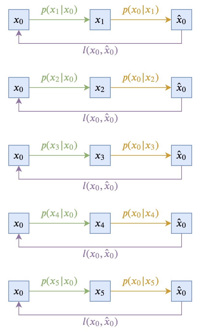Diagram of the forward process and training objective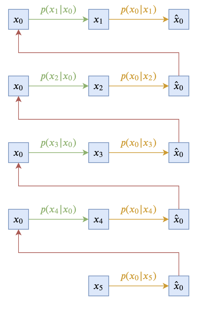Reverse process under the simplest choice

This minimal choice is theoretically sound, but in practice the results are usually not very good. That's because in this case $\boldsymbol{x}_{t-1}$ depends entirely on $\boldsymbol{x}_0$, and while $\boldsymbol{x}_0$ originally represents the true original sample, during the reverse process we can only approximately sample it through the approximate distribution $q(\boldsymbol{x}_0|\boldsymbol{x}_t)$, and $q(\boldsymbol{x}_0|\boldsymbol{x}_t)$ is usually not accurate enough — so the errors keep accumulating. Moreover, $p(\boldsymbol{x}_{t-1}|\boldsymbol{x}_0)$ carries noise during the sampling process, and this noise can severely corrupt the information about $\hat{\boldsymbol{x}}_0$ that was just estimated, degrading the generation quality.

Fortunately, in most cases, we can derive a new result based on this simple choice $p(\boldsymbol{x}_{t-1}|\boldsymbol{x}_t, \boldsymbol{x}_0) = p(\boldsymbol{x}_{t-1}|\boldsymbol{x}_0)$. From equation $\eqref{eq:re-param}$, we know that

\begin{equation}\begin{aligned} \boldsymbol{x}_{t-1} \sim p(\boldsymbol{x}_{t-1}|\boldsymbol{x}_0)\quad\Leftrightarrow&\,\quad\boldsymbol{x}_{t-1} = \boldsymbol{\mathcal{F}}_{t-1}(\boldsymbol{x}_0,\boldsymbol{\varepsilon}) \\ \boldsymbol{x}_t \sim p(\boldsymbol{x}_t|\boldsymbol{x}_0)\quad\Leftrightarrow&\,\quad\boldsymbol{x}_t = \boldsymbol{\mathcal{F}}_t(\boldsymbol{x}_0,\boldsymbol{\varepsilon}) \end{aligned}\end{equation}

Assuming $\boldsymbol{\mathcal{F}}_t(\boldsymbol{x}_0,\boldsymbol{\varepsilon})$ is invertible with respect to $\boldsymbol{\varepsilon}$, we can solve for $\boldsymbol{\varepsilon} = \boldsymbol{\mathcal{F}}_t^{-1}(\boldsymbol{x}_0,\boldsymbol{x}_t)$, and this solved-for $\boldsymbol{\varepsilon}$ can then be used to replace $\boldsymbol{\varepsilon}$ appearing in $\boldsymbol{\mathcal{F}}_{t-1}(\boldsymbol{x}_0,\boldsymbol{\varepsilon})$, giving

\begin{equation}\boldsymbol{x}_{t-1} = \boldsymbol{\mathcal{F}}_{t-1}(\boldsymbol{x}_0,\boldsymbol{\mathcal{F}}_t^{-1}(\boldsymbol{x}_0,\boldsymbol{x}_t))\end{equation}

which amounts to

\begin{equation}p(\boldsymbol{x}_{t-1}|\boldsymbol{x}_t, \boldsymbol{x}_0) = \delta\big(\boldsymbol{x}_{t-1} - \boldsymbol{\mathcal{F}}_{t-1}(\boldsymbol{x}_0,\boldsymbol{\mathcal{F}}_t^{-1}(\boldsymbol{x}_0,\boldsymbol{x}_t))\big)\end{equation}

being a design for $p(\boldsymbol{x}_{t-1}|\boldsymbol{x}_t, \boldsymbol{x}_0)$ that depends simultaneously on $\boldsymbol{x}_t, \boldsymbol{x}_0$. Here $\boldsymbol{x}_t$ offloads part of $\boldsymbol{x}_{t-1}$'s dependence on $\boldsymbol{x}_0$, and eliminates the noise, so that the "progress" made at each generation step can be stably accumulated. As a result, a reverse process using this design tends to perform better.

Furthermore, if $q(\boldsymbol{\varepsilon})$ is the standard normal distribution, we can obtain an even more general result, because by the additivity of normal distributions we have

\begin{equation}\boldsymbol{x}_{t-1} = \boldsymbol{\mathcal{F}}_{t-1}(\boldsymbol{x}_0,\boldsymbol{\varepsilon})\quad\Leftrightarrow\quad\boldsymbol{x}_{t-1} = \boldsymbol{\mathcal{F}}_{t-1}(\boldsymbol{x}_0,\sqrt{1 - \tilde{\sigma}_t^2}\boldsymbol{\varepsilon}_1 + \tilde{\sigma}_t \boldsymbol{\varepsilon}_2)\end{equation}

In this way, the $\boldsymbol{\varepsilon}$ solved from $\boldsymbol{x}_0,\boldsymbol{x}_t$ can be used to replace just one of $\boldsymbol{\varepsilon}_1$ or $\boldsymbol{\varepsilon}_2$, and the resulting sampling process for $p(\boldsymbol{x}_{t-1}|\boldsymbol{x}_t, \boldsymbol{x}_0)$ is

\begin{equation}\quad\boldsymbol{x}_{t-1} = \boldsymbol{\mathcal{F}}_{t-1}(\boldsymbol{x}_0,\sqrt{1 - \tilde{\sigma}_t^2}\boldsymbol{\mathcal{F}}_t^{-1}(\boldsymbol{x}_0,\boldsymbol{x}_t) + \tilde{\sigma}_t \boldsymbol{\varepsilon})\end{equation}

Discussion and Analysis

At this point, the theoretical framework of the unified diffusion model (UDM) has been fully constructed. In the next post, we'll go through some concrete examples showing how to derive existing diffusion model results from the UDM framework, and further obtain some new results. In this section, let's reflect on the reasoning of this whole post.

Having read through the whole post, I suspect quite a few readers are feeling a bit lost, because the result presented here is a unified framework distilled from everything the author has previously understood about diffusion models — the underlying techniques aren't especially difficult, but the logic isn't easy to untangle either. First, the goal of this post is to "design a unified theoretical framework for diffusion models," one capable of achieving the goals listed at the beginning of the post. The key to "design" is grasping the balance between "freedom" and "constraint": some parts can be chosen flexibly, while others carry constraints that cannot be violated.

If readers are already fairly familiar with existing generative diffusion models, they'll probably grasp that the essential idea of diffusion models is "learning to build by learning from destruction." In principle, the way we "destroy" can be chosen freely, while the "building" part is what needs to be learned. Of course, the way we destroy isn't actually completely unconstrained either — generally speaking, it must be a "progressive destruction," so that we can in turn learn a "progressive construction." In this way, we constructed the destruction process (the forward process) of equation $\eqref{eq:re-param}$, where $t$ describes the progress of the destruction, $\mathcal{F}$ can represent an arbitrary method of destruction, there's no particular restriction on the original data $\boldsymbol{x}_0$, and $\boldsymbol{\varepsilon}$ describes the randomness that may exist in the destruction process. In this way, we've established the most general possible destruction process.

As for construction, we first gave the decomposition $\eqref{eq:p-factor}$, which is an identity given by probability theory itself — we can understand it either as a constraint or as a guide. How did we know to think in the direction of equation $\eqref{eq:p-factor}$? Looking back, the forward process is a process of $\boldsymbol{x}_0\to \boldsymbol{x}_t$, so the reverse process should be tied to $\boldsymbol{x}_t\to \boldsymbol{x}_0$ as closely as possible, and from there we're naturally led to equation $\eqref{eq:p-factor}$.

The decomposition $\eqref{eq:p-factor}$ contains two parts. Of these, $p(\boldsymbol{x}_0|\boldsymbol{x}_t)$ is already quite clear — it's simply the probability of predicting $\boldsymbol{x}_0$ from $\boldsymbol{x}_t$, and this part clearly leaves no room for further simplification; it can only be directly modeled. The other part, $p(\boldsymbol{x}_{t-1}|\boldsymbol{x}_t, \boldsymbol{x}_0)$, falls under "free design": all that's required is that it be easy to sample from, and the "constraint" on it comes from an identity, $\eqref{eq:margin}$, which is again something given by probability theory itself. As for the subsequent process of designing $p(\boldsymbol{x}_{t-1}|\boldsymbol{x}_t, \boldsymbol{x}_0)$ under this constraint — that does require some real skill. There's no shortcut here; the author himself spent a long time thinking it through in conjunction with existing diffusion model work before finally untangling the process.

Overall, when designing a model, one must always keep clearly in mind what one wants ("freedom") and what limitations that desired thing is subject to ("constraint"). With "freedom" and "constraint" both made explicit, one should draw as much as possible on existing work and learned theoretical foundations, gradually converging toward the goal.

Summary

This post has constructed a new theoretical framework for diffusion models (Unified Diffusion Model, UDM), which in principle is able to encompass existing diffusion model results while allowing for more general diffusion mechanisms and data types. We'll introduce concrete examples in the next post.