Generative Diffusion Models Explained (VII): Optimal Diffusion Variance Estimation (Part 1)

生成扩散模型漫谈（七）：最优扩散方差估计（上） 苏剑林 · 2022-08-12 · Machine Learning optimization generative model DDPM diffusion

For generative diffusion models, a crucial question is how to choose the variance for the generation process, since different variances noticeably affect the quality of generation.

In Generative Diffusion Models Explained (II): DDPM = Autoregressive VAE, we mentioned that DDPM derived two usable results by assuming the data follows two particular special distributions; in Generative Diffusion Models Explained (IV): DDIM = A High-Level View of DDPM, DDIM instead adjusted the generation process by turning the variance into a hyperparameter, even allowing zero-variance generation—though DDIM with zero variance generally performs worse than DDPM with nonzero variance; Generative Diffusion Models Explained (V): The General SDE Framework shows that the forward and reverse SDEs should in principle share the same variance, but this only strictly holds when $\Delta t\to 0$; and Improved Denoising Diffusion Probabilistic Models proposed treating it as a trainable parameter to be learned, though this increases the difficulty of training.

So how should the variance of the generation process actually be set? Two papers from this year, Analytic-DPM: an Analytic Estimate of the Optimal Reverse Variance in Diffusion Probabilistic Models and Estimating the Optimal Covariance with Imperfect Mean in Diffusion Probabilistic Models, provide what amounts to a rather elegant answer to this question. Let's take a look at their results together. more

Uncertainty

As it happens, these two papers come from the same research group, and largely share the same authors. The first paper (abbreviated as Analytic-DPM) derives, building on DDIM, an analytic solution for the unconditional variance; the second paper (abbreviated as Extended-Analytic-DPM) relaxes the assumptions of the first paper and proposes a method for optimizing the conditional variance. This post first introduces the results of the first paper.

In Generative Diffusion Models Explained (IV): DDIM = A High-Level View of DDPM, we derived that for a given $p(\boldsymbol{x}_t|\boldsymbol{x}_0) = \mathcal{N}(\boldsymbol{x}_t;\bar{\alpha}_t \boldsymbol{x}_0,\bar{\beta}_t^2 \boldsymbol{I})$, the general solution for the corresponding $p(\boldsymbol{x}_{t-1}|\boldsymbol{x}_t, \boldsymbol{x}_0)$ is

\begin{equation}p(\boldsymbol{x}_{t-1}|\boldsymbol{x}_t, \boldsymbol{x}_0) = \mathcal{N}\left(\boldsymbol{x}_{t-1}; \frac{\sqrt{\bar{\beta}_{t-1}^2 - \sigma_t^2}}{\bar{\beta}_t} \boldsymbol{x}_t + \gamma_t \boldsymbol{x}_0, \sigma_t^2 \boldsymbol{I}\right)\end{equation}

where $\gamma_t = \bar{\alpha}_{t-1} - \frac{\bar{\alpha}_t\sqrt{\bar{\beta}_{t-1}^2 - \sigma_t^2}}{\bar{\beta}_t}$, and $\sigma_t$ is the tunable standard-deviation parameter. In DDIM, the subsequent processing step is: use $\bar{\boldsymbol{\mu}}(\boldsymbol{x}_t)$ to estimate $\boldsymbol{x}_0$, and then take

\begin{equation}p(\boldsymbol{x}_{t-1}|\boldsymbol{x}_t) \approx p(\boldsymbol{x}_{t-1}|\boldsymbol{x}_t, \boldsymbol{x}_0=\bar{\boldsymbol{\mu}}(\boldsymbol{x}_t))\end{equation}

However, from a Bayesian perspective, this is quite improper, because predicting $\boldsymbol{x}_0$ from $\boldsymbol{x}_t$ can never be entirely accurate—it carries a certain degree of uncertainty, and therefore we ought to describe it with a probability distribution rather than a deterministic function. In fact, we strictly have

\begin{equation}p(\boldsymbol{x}_{t-1}|\boldsymbol{x}_t) = \int p(\boldsymbol{x}_{t-1}|\boldsymbol{x}_t, \boldsymbol{x}_0)p(\boldsymbol{x}_0|\boldsymbol{x}_t)d\boldsymbol{x}_0\end{equation}

The exact $p(\boldsymbol{x}_0|\boldsymbol{x}_t)$ is generally unobtainable, but here we only need a crude approximation, so we approximate it with a normal distribution $\mathcal{N}(\boldsymbol{x}_0;\bar{\boldsymbol{\mu}}(\boldsymbol{x}_t),\bar{\sigma}_t^2\boldsymbol{I})$ (we'll discuss how to approximate it later). With this approximate distribution in hand, we can write

\begin{equation}\begin{aligned} \boldsymbol{x}_{t-1} =&\, \frac{\sqrt{\bar{\beta}_{t-1}^2 - \sigma_t^2}}{\bar{\beta}_t}\boldsymbol{x}_t + \gamma_t \boldsymbol{x}_0 + \sigma_t\boldsymbol{\varepsilon}_1 \\ \approx&\, \frac{\sqrt{\bar{\beta}_{t-1}^2 - \sigma_t^2}}{\bar{\beta}_t}\boldsymbol{x}_t + \gamma_t \big(\bar{\boldsymbol{\mu}}(\boldsymbol{x}_t) + \bar{\sigma}_t \boldsymbol{\varepsilon}_2\big) + \sigma_t\boldsymbol{\varepsilon}_1 \\ =&\, \left(\frac{\sqrt{\bar{\beta}_{t-1}^2 - \sigma_t^2}}{\bar{\beta}_t}\boldsymbol{x}_t + \gamma_t \bar{\boldsymbol{\mu}}(\boldsymbol{x}_t)\right) + \underbrace{\big(\sigma_t\boldsymbol{\varepsilon}_1 + \gamma_t\bar{\sigma}_t \boldsymbol{\varepsilon}_2\big)}_{ \sim \sqrt{\sigma_t^2 + \gamma_t^2\bar{\sigma}_t^2}\boldsymbol{\varepsilon}} \\ \end{aligned}\end{equation}

where $\boldsymbol{\varepsilon}_1,\boldsymbol{\varepsilon}_2,\boldsymbol{\varepsilon}\sim\mathcal{N}(\boldsymbol{0},\boldsymbol{I})$. As we can see, $p(\boldsymbol{x}_{t-1}|\boldsymbol{x}_t)$ is more closely approximated by a normal distribution with mean $\frac{\sqrt{\bar{\beta}_{t-1}^2 - \sigma_t^2}}{\bar{\beta}_t}\boldsymbol{x}_t + \gamma_t \bar{\boldsymbol{\mu}}(\boldsymbol{x}_t)$ and covariance $\left(\sigma_t^2 + \gamma_t^2\bar{\sigma}_t^2\right)\boldsymbol{I}$, where the mean is consistent with the previous result, but the variance now has an extra term $\gamma_t^2\bar{\sigma}_t^2$. Consequently, even when $\sigma_t=0$, the corresponding variance is not zero. This extra term is precisely the correction to the optimal variance proposed in the first paper.

Mean Optimization

Now let's discuss how to use $\mathcal{N}(\boldsymbol{x}_0;\bar{\boldsymbol{\mu}}(\boldsymbol{x}_t),\bar{\sigma}_t^2\boldsymbol{I})$ to approximate the true $p(\boldsymbol{x}_0|\boldsymbol{x}_t)$—in plain terms, how to find the mean and covariance of $p(\boldsymbol{x}_0|\boldsymbol{x}_t)$.

For the mean $\bar{\boldsymbol{\mu}}(\boldsymbol{x}_t)$, since it depends on $\boldsymbol{x}_t$, we need a model to fit it, and training a model requires a loss function. Using

\begin{equation}\mathbb{E}_{\boldsymbol{x}}[\boldsymbol{x}] = \mathop{\text{argmin}}_{\boldsymbol{\mu}}\mathbb{E}_{\boldsymbol{x}}\left[\Vert \boldsymbol{x} - \boldsymbol{\mu}\Vert^2\right]\label{eq:mean-opt}\end{equation}

we obtain

\begin{equation}\begin{aligned} \bar{\boldsymbol{\mu}}(\boldsymbol{x}_t) =&\,\mathbb{E}_{\boldsymbol{x}_0\sim p(\boldsymbol{x}_0|\boldsymbol{x}_t)}[\boldsymbol{x}_0] \\[5pt] =&\, \mathop{\text{argmin}}_{\boldsymbol{\mu}}\mathbb{E}_{\boldsymbol{x}_0\sim p(\boldsymbol{x}_0|\boldsymbol{x}_t)}\left[\Vert \boldsymbol{x}_0 - \boldsymbol{\mu}\Vert^2\right] \\ =&\, \mathop{\text{argmin}}_{\boldsymbol{\mu}(\boldsymbol{x}_t)}\mathbb{E}_{\boldsymbol{x}_t\sim p(\boldsymbol{x}_t)}\mathbb{E}_{\boldsymbol{x}_0\sim p(\boldsymbol{x}_0|\boldsymbol{x}_t)}\left[\left\Vert \boldsymbol{x}_0 - \boldsymbol{\mu}(\boldsymbol{x}_t)\right\Vert^2\right] \\ =&\, \mathop{\text{argmin}}_{\boldsymbol{\mu}(\boldsymbol{x}_t)}\mathbb{E}_{\boldsymbol{x}_0\sim \tilde{p}(\boldsymbol{x}_0)}\mathbb{E}_{\boldsymbol{x}_t\sim p(\boldsymbol{x}_t|\boldsymbol{x}_0)}\left[\left\Vert \boldsymbol{x}_0 - \boldsymbol{\mu}(\boldsymbol{x}_t)\right\Vert^2\right] \\ \end{aligned}\label{eq:loss-1}\end{equation}

This is the loss function used to train $\bar{\boldsymbol{\mu}}(\boldsymbol{x}_t)$. If we introduce the same parameterization as before,

\begin{equation}\bar{\boldsymbol{\mu}}(\boldsymbol{x}_t) = \frac{1}{\bar{\alpha}_t}\left(\boldsymbol{x}_t - \bar{\beta}_t \boldsymbol{\epsilon}_{\boldsymbol{\theta}}(\boldsymbol{x}_t, t)\right)\label{eq:bar-mu}\end{equation}

we recover the familiar DDPM training loss form $\left\Vert\boldsymbol{\varepsilon} - \boldsymbol{\epsilon}_{\boldsymbol{\theta}}(\bar{\alpha}_t \boldsymbol{x}_0 + \bar{\beta}_t \boldsymbol{\varepsilon}, t)\right\Vert^2$. The result for mean optimization is thus consistent with what we had before—nothing changes here.

Variance Estimation 1

Similarly, by definition, the covariance matrix should be

\begin{equation}\begin{aligned} \boldsymbol{\Sigma}(\boldsymbol{x}_t)=&\, \mathbb{E}_{\boldsymbol{x}_0\sim p(\boldsymbol{x}_0|\boldsymbol{x}_t)}\left[\left(\boldsymbol{x}_0 - \bar{\boldsymbol{\mu}}(\boldsymbol{x}_t)\right)\left(\boldsymbol{x}_0 - \bar{\boldsymbol{\mu}}(\boldsymbol{x}_t)\right)^{\top}\right] \\ =&\, \mathbb{E}_{\boldsymbol{x}_0\sim p(\boldsymbol{x}_0|\boldsymbol{x}_t)}\left[\left((\boldsymbol{x}_0 - \boldsymbol{\mu}) - (\bar{\boldsymbol{\mu}}(\boldsymbol{x}_t) - \boldsymbol{\mu})\right)\left((\boldsymbol{x}_0 - \boldsymbol{\mu}) - (\bar{\boldsymbol{\mu}}(\boldsymbol{x}_t) - \boldsymbol{\mu})\right)^{\top}\right] \\ =&\, \mathbb{E}_{\boldsymbol{x}_0\sim p(\boldsymbol{x}_0|\boldsymbol{x}_t)}\left[(\boldsymbol{x}_0 - \boldsymbol{\mu}_0)(\boldsymbol{x}_0 - \boldsymbol{\mu}_0)^{\top}\right] - (\bar{\boldsymbol{\mu}}(\boldsymbol{x}_t) - \boldsymbol{\mu}_0)(\bar{\boldsymbol{\mu}}(\boldsymbol{x}_t) - \boldsymbol{\mu}_0)^{\top}\\ \end{aligned}\label{eq:var-expand}\end{equation}

where $\boldsymbol{\mu}_0$ can be any constant vector, reflecting the translation invariance of covariance.

The above expression estimates the full covariance matrix, but that isn't quite what we want, because here we want to use $\mathcal{N}(\boldsymbol{x}_0;\bar{\boldsymbol{\mu}}(\boldsymbol{x}_t),\bar{\sigma}_t^2\boldsymbol{I})$ to approximate $p(\boldsymbol{x}_0|\boldsymbol{x}_t)$, where the designed covariance matrix is $\bar{\sigma}_t^2\boldsymbol{I}$, which has two distinguishing features:

1. Independence from $\boldsymbol{x}_t$: to eliminate the dependence on $\boldsymbol{x}_t$, we average over all $\boldsymbol{x}_t$, i.e. $\boldsymbol{\Sigma}_t = \mathbb{E}_{\boldsymbol{x}_t\sim p(\boldsymbol{x}_t)}[\boldsymbol{\Sigma}(\boldsymbol{x}_t)]$;
2. A multiple of the identity matrix: this means we only need to consider the diagonal entries, and we average over them, i.e. $\bar{\sigma}_t^2 = \text{Tr}(\boldsymbol{\Sigma}_t)/d$, where $d=\dim(\boldsymbol{x})$.

This gives us

\begin{equation}\begin{aligned} \bar{\sigma}_t^2 =&\, \mathbb{E}_{\boldsymbol{x}_t\sim p(\boldsymbol{x}_t)}\mathbb{E}_{\boldsymbol{x}_0\sim p(\boldsymbol{x}_0|\boldsymbol{x}_t)}\left[\frac{\Vert\boldsymbol{x}_0 - \boldsymbol{\mu}_0\Vert^2}{d}\right] - \mathbb{E}_{\boldsymbol{x}_t\sim p(\boldsymbol{x}_t)}\left[\frac{\Vert\bar{\boldsymbol{\mu}}(\boldsymbol{x}_t) - \boldsymbol{\mu}_0\Vert^2}{d}\right] \\ =&\, \frac{1}{d}\mathbb{E}_{\boldsymbol{x}_0\sim \tilde{p}(\boldsymbol{x}_0)}\mathbb{E}_{\boldsymbol{x}_t\sim p(\boldsymbol{x}_t|\boldsymbol{x}_0)}\left[\Vert\boldsymbol{x}_0 - \boldsymbol{\mu}_0\Vert^2\right] - \frac{1}{d}\mathbb{E}_{\boldsymbol{x}_t\sim p(\boldsymbol{x}_t)}\left[\Vert\bar{\boldsymbol{\mu}}(\boldsymbol{x}_t) - \boldsymbol{\mu}_0\Vert^2\right] \\ =&\, \frac{1}{d}\mathbb{E}_{\boldsymbol{x}_0\sim \tilde{p}(\boldsymbol{x}_0)}\left[\Vert\boldsymbol{x}_0 - \boldsymbol{\mu}_0\Vert^2\right] - \frac{1}{d}\mathbb{E}_{\boldsymbol{x}_t\sim p(\boldsymbol{x}_t)}\left[\Vert\bar{\boldsymbol{\mu}}(\boldsymbol{x}_t) - \boldsymbol{\mu}_0\Vert^2\right] \\ \end{aligned}\label{eq:var-1}\end{equation}

This is an analytic form for $\bar{\sigma}_t^2$ that I've worked out myself; once $\bar{\boldsymbol{\mu}}(\boldsymbol{x}_t)$ has finished training, this can be approximated by sampling a batch of $\boldsymbol{x}_0$ and $\boldsymbol{x}_t$.

In particular, if we take $\boldsymbol{\mu}_0=\mathbb{E}_{\boldsymbol{x}_0\sim \tilde{p}(\boldsymbol{x}_0)}[\boldsymbol{x}_0]$, this can be written neatly as

\begin{equation}\bar{\sigma}_t^2 = \mathbb{V}ar[\boldsymbol{x}_0] - \frac{1}{d}\mathbb{E}_{\boldsymbol{x}_t\sim p(\boldsymbol{x}_t)}\left[\Vert\bar{\boldsymbol{\mu}}(\boldsymbol{x}_t) - \boldsymbol{\mu}_0\Vert^2\right]\end{equation}

Here $\mathbb{V}ar[\boldsymbol{x}_0]$ is the pixel-level variance over the entire training set $\boldsymbol{x}_0$. If every pixel value of $\boldsymbol{x}_0$ lies within the interval $[a,b]$, then its variance clearly cannot exceed $\left(\frac{b-a}{2}\right)^2$, giving us the inequality

\begin{equation}\bar{\sigma}_t^2 \leq \mathbb{V}ar[\boldsymbol{x}_0] \leq \left(\frac{b-a}{2}\right)^2\end{equation}

Variance Estimation 2

The solution just given is the one I find more intuitive, but the original Analytic-DPM paper gives a slightly different solution—one that I personally find less intuitive. By substituting into equation $\eqref{eq:bar-mu}$, we can obtain:

\begin{equation}\begin{aligned} \boldsymbol{\Sigma}(\boldsymbol{x}_t)=&\, \mathbb{E}_{\boldsymbol{x}_0\sim p(\boldsymbol{x}_0|\boldsymbol{x}_t)}\left[\left(\boldsymbol{x}_0 - \bar{\boldsymbol{\mu}}(\boldsymbol{x}_t)\right)\left(\boldsymbol{x}_0 - \bar{\boldsymbol{\mu}}(\boldsymbol{x}_t)\right)^{\top}\right] \\ =&\, \mathbb{E}_{\boldsymbol{x}_0\sim p(\boldsymbol{x}_0|\boldsymbol{x}_t)}\left[\left(\left(\boldsymbol{x}_0 - \frac{\boldsymbol{x}_t}{\bar{\alpha}_t}\right) + \frac{\bar{\beta}_t}{\bar{\alpha}_t} \boldsymbol{\epsilon}_{\boldsymbol{\theta}}(\boldsymbol{x}_t, t)\right)\left(\left(\boldsymbol{x}_0 - \frac{\boldsymbol{x}_t}{\bar{\alpha}_t}\right) + \frac{\bar{\beta}_t}{\bar{\alpha}_t} \boldsymbol{\epsilon}_{\boldsymbol{\theta}}(\boldsymbol{x}_t, t)\right)^{\top}\right] \\ =&\, \mathbb{E}_{\boldsymbol{x}_0\sim p(\boldsymbol{x}_0|\boldsymbol{x}_t)}\left[\left(\boldsymbol{x}_0 - \frac{\boldsymbol{x}_t}{\bar{\alpha}_t}\right)\left(\boldsymbol{x}_0 - \frac{\boldsymbol{x}_t}{\bar{\alpha}_t}\right)^{\top}\right] - \frac{\bar{\beta}_t^2}{\bar{\alpha}_t^2} \boldsymbol{\epsilon}_{\boldsymbol{\theta}}(\boldsymbol{x}_t, t)\boldsymbol{\epsilon}_{\boldsymbol{\theta}}(\boldsymbol{x}_t, t)^{\top}\\ =&\, \frac{1}{\bar{\alpha}_t^2}\mathbb{E}_{\boldsymbol{x}_0\sim p(\boldsymbol{x}_0|\boldsymbol{x}_t)}\left[\left(\boldsymbol{x}_t - \bar{\alpha}_t\boldsymbol{x}_0\right)\left(\boldsymbol{x}_t - \bar{\alpha}_t\boldsymbol{x}_0\right)^{\top}\right] - \frac{\bar{\beta}_t^2}{\bar{\alpha}_t^2} \boldsymbol{\epsilon}_{\boldsymbol{\theta}}(\boldsymbol{x}_t, t)\boldsymbol{\epsilon}_{\boldsymbol{\theta}}(\boldsymbol{x}_t, t)^{\top}\\ \end{aligned}\end{equation}

If we now average both sides over $\boldsymbol{x}_t\sim p(\boldsymbol{x}_t)$, we get

\begin{equation}\begin{aligned} &\,\mathbb{E}_{\boldsymbol{x}_t\sim p(\boldsymbol{x}_t)}\mathbb{E}_{\boldsymbol{x}_0\sim p(\boldsymbol{x}_0|\boldsymbol{x}_t)}\left[\left(\boldsymbol{x}_t - \bar{\alpha}_t\boldsymbol{x}_0\right)\left(\boldsymbol{x}_t - \bar{\alpha}_t\boldsymbol{x}_0\right)^{\top}\right] \\ =&\, \mathbb{E}_{\boldsymbol{x}_0\sim \tilde{p}(\boldsymbol{x}_0)}\mathbb{E}_{\boldsymbol{x}_t\sim p(\boldsymbol{x}_t|\boldsymbol{x}_0)}\left[\left(\boldsymbol{x}_t - \bar{\alpha}_t\boldsymbol{x}_0\right)\left(\boldsymbol{x}_t - \bar{\alpha}_t\boldsymbol{x}_0\right)^{\top}\right] \end{aligned}\end{equation}

Remember that $p(\boldsymbol{x}_t|\boldsymbol{x}_0) = \mathcal{N}(\boldsymbol{x}_t;\bar{\alpha}_t \boldsymbol{x}_0,\bar{\beta}_t^2 \boldsymbol{I})$, so $\bar{\alpha}_t \boldsymbol{x}_0$ is in fact the mean of $p(\boldsymbol{x}_t|\boldsymbol{x}_0)$, meaning $\mathbb{E}_{\boldsymbol{x}_t\sim p(\boldsymbol{x}_t|\boldsymbol{x}_0)}\left[\left(\boldsymbol{x}_t - \bar{\alpha}_t\boldsymbol{x}_0\right)\left(\boldsymbol{x}_t - \bar{\alpha}_t\boldsymbol{x}_0\right)^{\top}\right]$ is essentially computing the covariance matrix of the mean of $p(\boldsymbol{x}_t|\boldsymbol{x}_0)$, and the result is obviously $\bar{\beta}_t^2 \boldsymbol{I}$, so

\begin{equation}\mathbb{E}_{\boldsymbol{x}_0\sim \tilde{p}(\boldsymbol{x}_0)}\mathbb{E}_{\boldsymbol{x}_t\sim p(\boldsymbol{x}_t|\boldsymbol{x}_0)}\left[\left(\boldsymbol{x}_t - \bar{\alpha}_t\boldsymbol{x}_0\right)\left(\boldsymbol{x}_t - \bar{\alpha}_t\boldsymbol{x}_0\right)^{\top}\right] = \mathbb{E}_{\boldsymbol{x}_0\sim \tilde{p}(\boldsymbol{x}_0)}\left[\bar{\beta}_t^2 \boldsymbol{I}\right] = \bar{\beta}_t^2 \boldsymbol{I} \end{equation}

which gives

\begin{equation} \boldsymbol{\Sigma}_t = \mathbb{E}_{\boldsymbol{x}_t\sim p(\boldsymbol{x}_t)}[\boldsymbol{\Sigma}(\boldsymbol{x}_t)] = \frac{\bar{\beta}_t^2}{\bar{\alpha}_t^2}\left(\boldsymbol{I} - \mathbb{E}_{\boldsymbol{x}_t\sim p(\boldsymbol{x}_t)}\left[ \boldsymbol{\epsilon}_{\boldsymbol{\theta}}(\boldsymbol{x}_t, t)\boldsymbol{\epsilon}_{\boldsymbol{\theta}}(\boldsymbol{x}_t, t)^{\top}\right]\right)\end{equation}

Taking the trace of both sides and dividing by $d$, we obtain

\begin{equation}\bar{\sigma}_t^2 = \frac{\bar{\beta}_t^2}{\bar{\alpha}_t^2}\left(1 - \frac{1}{d}\mathbb{E}_{\boldsymbol{x}_t\sim p(\boldsymbol{x}_t)}\left[ \Vert\boldsymbol{\epsilon}_{\boldsymbol{\theta}}(\boldsymbol{x}_t, t)\Vert^2\right]\right)\leq \frac{\bar{\beta}_t^2}{\bar{\alpha}_t^2}\label{eq:var-2}\end{equation}

This yields another estimate and upper bound—this is the original result from Analytic-DPM.

Experimental Results

The experiments in the original paper show that the variance correction introduced by Analytic-DPM produces a fairly noticeable improvement mainly when the number of diffusion generation steps is small, which makes it particularly meaningful for accelerating diffusion models:

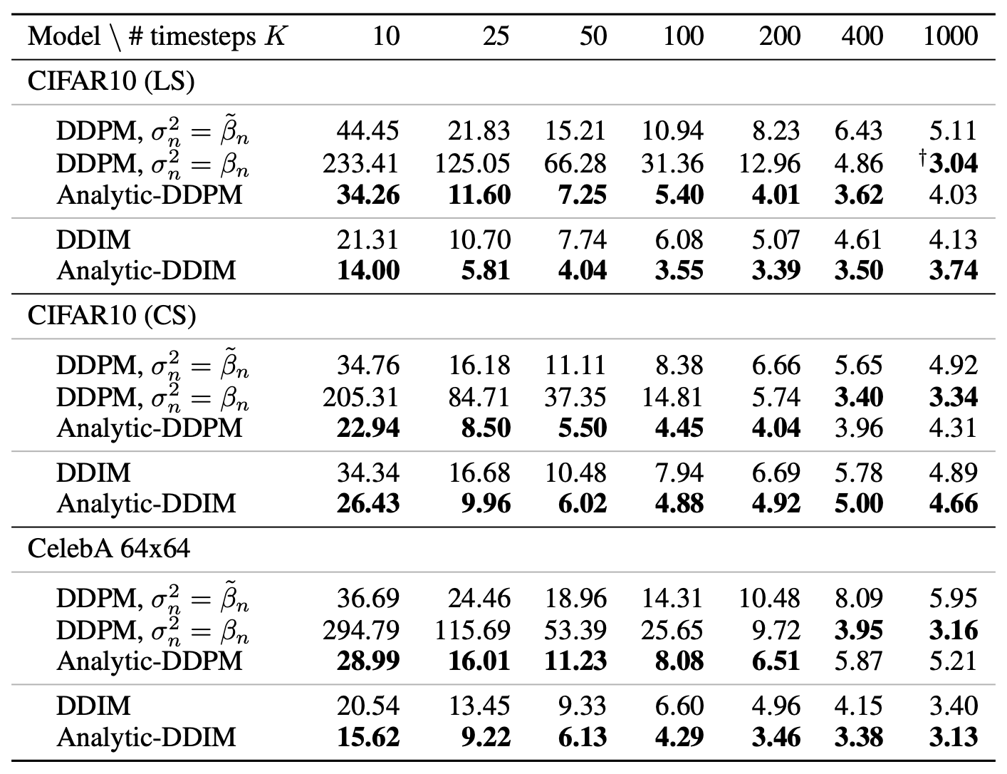Analytic-DPM mainly shows a noticeable improvement when the number of diffusion steps is small

I also tried applying the Analytic-DPM correction to my own previously implemented code. The reference code is here:

GitHub: https://github.com/bojone/Keras-DDPM/blob/main/adpm.py

When the number of diffusion steps is $10$, the comparison between DDPM and Analytic-DDPM is shown below:

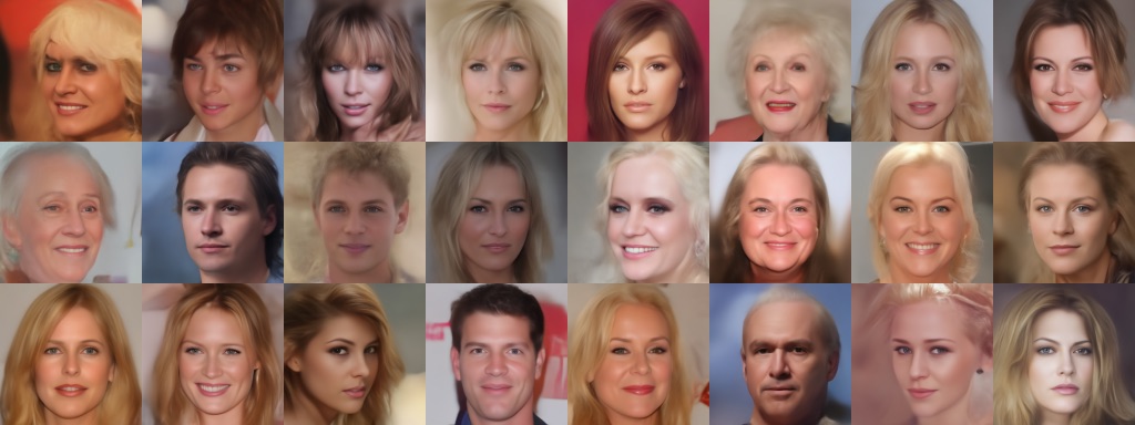DDPM generation results with 10 diffusion steps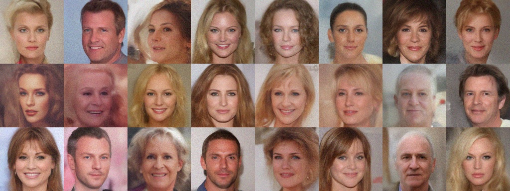Analytic-DDPM generation results with 10 diffusion steps

As we can see, when the number of diffusion steps is small, DDPM's generated results look rather smooth, with something of a "heavily airbrushed" quality; by comparison, Analytic-DDPM's results look somewhat more realistic, though this also introduces extra noise. In terms of evaluation metrics, Analytic-DDPM performs somewhat better.

Nitpicking

At this point we've finished introducing Analytic-DPM. The derivation carries a bit of technical cleverness, but isn't overly complicated—at least the underlying logic is fairly clear. If readers still find it hard to follow, feel free to go look at the original paper's appendix, which completes the derivation across seven pages and thirteen lemmas—after seeing that, I suspect you'll come to appreciate just how friendly this post's derivation is, ha!

To be fair, as far as being the first to obtain this analytic solution for the variance goes, I'm genuinely impressed by the original authors' insight. But I have to say that, with the benefit of hindsight, Analytic-DPM takes something of a "roundabout path" in both its derivation and its results—it comes across as "overly convoluted" and "overly clever," in a way that doesn't feel especially illuminating. One of the most obvious symptoms is that the original paper expresses all its results in terms of $\nabla_{\boldsymbol{x}_t}\log p(\boldsymbol{x}_t)$, which brings three problems: first, it makes the derivation process particularly unintuitive, leaving one wondering "how did they even think of this?"; second, it requires readers to have additional background in score matching results, raising the barrier to understanding; and finally, when it comes to actually implementing things, $\nabla_{\boldsymbol{x}_t}\log p(\boldsymbol{x}_t)$ has to be converted back to $\bar{\boldsymbol{\mu}}(\boldsymbol{x}_t)$ or $\boldsymbol{\epsilon}_{\boldsymbol{\theta}}(\boldsymbol{x}_t, t)$ anyway—an extra unnecessary detour.

The starting point of this post's derivation is that we are estimating the parameters of a normal distribution, and for a normal distribution, the method-of-moments estimate coincides with the maximum likelihood estimate—so we can simply estimate the corresponding mean and variance directly. As a result, there's no need to force things into a form aligned with $\nabla_{\boldsymbol{x}_t}\log p(\boldsymbol{x}_t)$ or score matching, since it's quite clear that Analytic-DPM's baseline model is DDIM, and DDIM itself was never derived from a score-matching starting point. Adding a connection to score matching doesn't benefit either the theory or the experiments. Aligning directly with $\bar{\boldsymbol{\mu}}(\boldsymbol{x}_t)$ or $\boldsymbol{\epsilon}_{\boldsymbol{\theta}}(\boldsymbol{x}_t, t)$ is more intuitive in form, and also converts more easily into experimental form.

Summary

This post shared the results on optimal diffusion-model variance estimation from the paper Analytic-DPM, which gives a directly usable analytic formula for the optimal variance estimate, letting us apply it to improve generation quality without needing to retrain anything. I simplified the original paper's derivation using my own approach, and carried out some simple experimental verification.