WGAN New Approach: Enforcing the L-constraint via Gradient Normalization

WGAN新方案：通过梯度归一化来实现L约束 苏剑林 · 2021-11-15 · Machine Learning unsupervised GAN generative model

At present, the mainstream implementations of WGAN include Weight Clipping, Spectral Normalization, and Gradient Penalty. This post introduces a new implementation scheme: Gradient Normalization. This scheme comes from two rather interesting papers, namely 《Gradient Normalization for Generative Adversarial Networks》 and 《GraN-GAN: Piecewise Gradient Normalization for Generative Adversarial Networks》.

What's interesting about them? As you can tell from the titles, these two papers should be highly overlapping, and perhaps even by the same authors. But in fact, they are two papers from different teams, produced at roughly the same time — one was accepted to ICCV, the other to WACV — and they arrive at essentially the same solution based on the same assumptions. The degree of overlap is so high that I kept thinking they were the same paper. Coincidences really are everywhere~ more

Background Recap

We've covered WGAN many times before, e.g. in 《The Art of Mutual Sparring: Getting Straight to WGAN-GP》 and 《From Wasserstein Distance and Duality Theory to WGAN》, so we won't repeat the details here. Briefly, the iterative form of WGAN is:

\begin{equation}\min_G \max_{\Vert D\Vert_{L}\leq 1} \mathbb{E}_{x\sim p(x)}\left[D(x)\right] - \mathbb{E}_{z\sim q(z)}\left[D(G(z))\right]\end{equation}

The key point here is that the discriminator $D$ is a constrained optimization problem: it needs to satisfy the L-constraint $\Vert D\Vert_{L}\leq 1$ during optimization. So the difficulty in implementing WGAN lies in how to inject this constraint into $D$.

Let's review the basics: if there exists a constant $C$ such that any $x,y$ in the domain satisfies $|f(x)-f(y)|\leq C\Vert x - y\Vert$, then we say that $f(x)$ satisfies the Lipschitz constraint (L-constraint), and the minimal value of $C$ is called the Lipschitz constant (L-constant), denoted $\Vert f\Vert_{L}$. So for the WGAN discriminator, two things need to be accomplished: 1) $D$ must satisfy the L-constraint; 2) the L-constant must not exceed 1.

In fact, our current mainstream neural network models are all of the form "linear combination + activation function," and the mainstream activation functions are "near-linear" — e.g. ReLU, LeakyReLU, SoftPlus — whose derivatives never exceed 1 in absolute value. So current mainstream models actually already satisfy the L-constraint, and the key issue is just how to keep the L-constant from exceeding 1 — though it doesn't really have to be exactly 1; it's enough to guarantee it stays below some fixed constant.

Overview of the Approach

Weight Clipping and Spectral Normalization share a similar idea: both constrain the parameters so that the L-constant of each layer of the model is bounded, and hence the overall L-constant is bounded too. Gradient Penalty, on the other hand, notices that a sufficient condition for $\Vert D\Vert_{L}\leq 1$ is $\Vert \nabla_x D(x)\Vert \leq 1$, and so it imposes a "soft constraint" via the penalty term $(\Vert \nabla_x D(x)\Vert - 1)^2$.

The Gradient Normalization introduced in this post is based on the same sufficient condition. It uses the gradient to transform $D(x)$ into $\hat{D}(x)$, so that it automatically satisfies $\Vert\nabla_x \hat{D}(x)\Vert \leq 1$. Specifically, we usually use ReLU or LeakyReLU as the activation function, under which $D(x)$ is in fact a "piecewise linear function." This means that, apart from at the boundaries, $D(x)$ is locally a linear function within each continuous region, and correspondingly $\nabla_x D(x)$ is a constant vector locally.

So Gradient Normalization aims to set $\hat{D}(x)=D(x)/\Vert \nabla_x D(x)\Vert$, which gives us

\begin{equation}\Vert\nabla_x \hat{D}(x)\Vert = \left\Vert \nabla_x \left(\frac{D(x)}{\Vert \nabla_x D(x)\Vert}\right)\right\Vert=\left\Vert \frac{\nabla_x D(x)}{\Vert \nabla_x D(x)\Vert}\right\Vert=1\end{equation}

Of course, this may run into division-by-zero issues, so the two papers propose different solutions. The first (the ICCV paper) directly adds $|D(x)|$ to the denominator as well, which incidentally also guarantees boundedness of the function:

\begin{equation} \hat{D}(x) = \frac{D(x)}{\Vert \nabla_x D(x)\Vert + |D(x)|}\in [-1,1]\end{equation}

The second (the WACV paper) takes the more straightforward approach of simply adding $\epsilon$:

\begin{equation} \hat{D}(x) = \frac{D(x)\cdot \Vert \nabla_x D(x)\Vert}{\Vert \nabla_x D(x)\Vert^2 + \epsilon}\end{equation}

The second paper also mentions having tried $\hat{D}(x)=D(x)/(\Vert \nabla_x D(x)\Vert+\epsilon)$, which performed slightly worse but was roughly comparable.

Experimental Results

Let's first look at the experimental results. Naturally, since both papers were accepted at top conferences, the results are certainly positive. Some of the results are shown below:

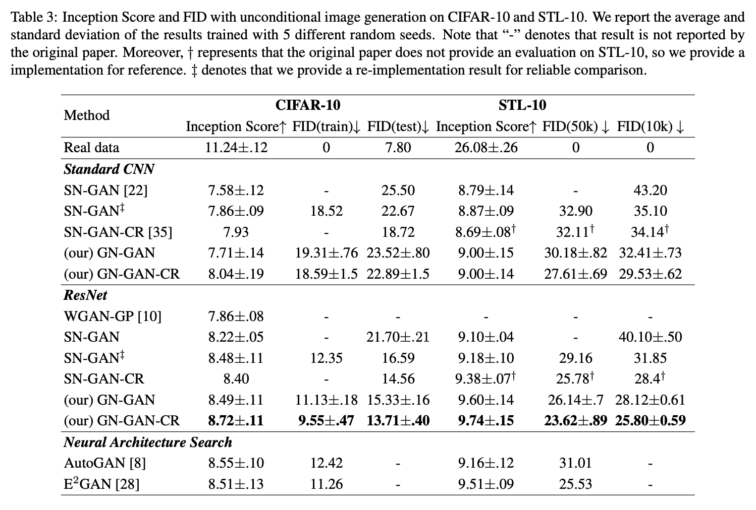Table of experimental results from the ICCV paper

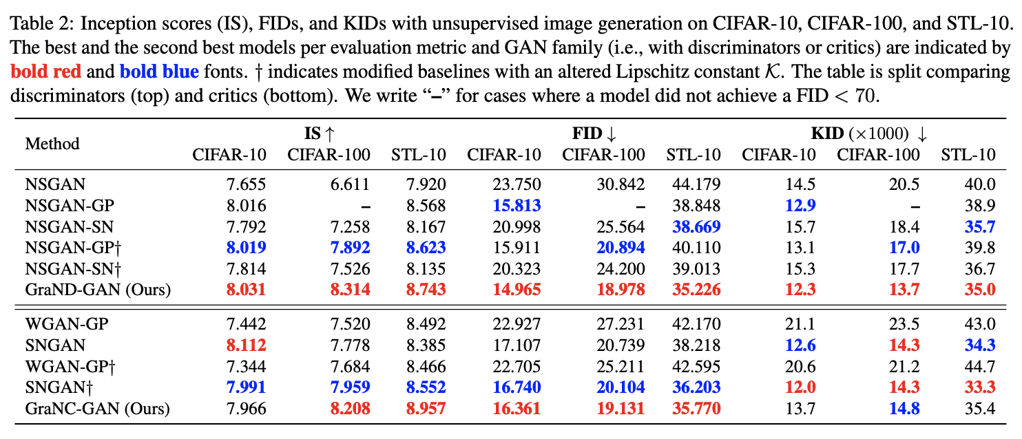Table of experimental results from the WACV paper

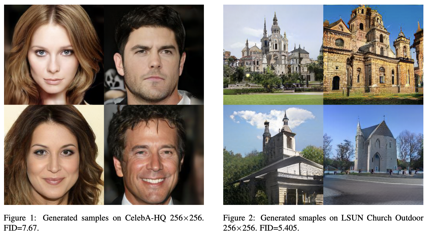Generated samples demonstrated in the ICCV paper

Lingering Questions

The results look good, the theory seems sound, and the work has been recognized by two top conferences at once — it certainly seems like solid work. However, my confusion is just getting started.

The most important issue with this work is this: if we go along with the piecewise-linear-function assumption, then although the gradient of $D(x)$ is locally constant, globally it is discontinuous (if the gradient were globally continuous and constant, then the function would be linear rather than piecewise linear). Yet $D(x)$ itself is a continuous function, so $\hat{D}(x)=D(x)/\Vert \nabla_x D(x)\Vert$ is a continuous function divided by a discontinuous one — and the result is a discontinuous function!

So here's the problem: it seems quite astonishing that a discontinuous function can serve as a discriminator. Note that this discontinuity isn't just at a few isolated boundary points — it's a discontinuity between two regions, so it's not something that can be brushed aside as negligible. On Reddit, other readers have raised the same question, but so far the authors haven't offered a satisfactory explanation (see the link).

Another issue: if the piecewise-linear-function assumption really holds, then using $\hat{D}(x)=\left\langle \frac{\nabla_x D(x)}{\Vert \nabla_x D(x)\Vert}, x\right\rangle$ directly as the discriminator ought, in theory, to be equivalent. But in my own experiments, using $\hat{D}(x)$ this way performs extremely poorly. So one possibility is that Gradient Normalization is indeed effective, but the reason it works isn't as simple as the analysis in these two papers suggests — perhaps there's a more complex mechanism at play that we haven't yet identified. Alternatively, it may be that our understanding of GANs is still far from adequate — that is, the requirements we place on discriminator continuity and so on may be quite different from what we currently believe.

Lastly, in my own experiments, Gradient Normalization performed worse than Gradient Penalty. And while Gradient Penalty only requires second-order gradients when training the discriminator, Gradient Normalization requires second-order gradients for training both the generator and the discriminator — so its speed is noticeably slower, and its memory footprint is noticeably larger. So from my personal hands-on experience, Gradient Normalization isn't a particularly friendly scheme to work with.

Summary

This post introduced a new scheme for implementing WGAN — Gradient Normalization. The scheme is fairly simple in form, and the results reported in the papers are quite good, but personally I think there remain quite a few points worth questioning.