The Art of Mutual Sparring: From Scratch Straight to WGAN-GP
Preface
GAN, short for Generative Adversarial Nets, is called "生成对抗式网络" in Chinese. For GAN, the most common explanation is the "forger–detective" story, like a forger and a detective in the art world. At first, neither the forger nor the detective is very skilled, and the detective can easily spot the fakes produced by the forger. But as the forger's craft improves, their fakes start to fool the detective; or, as the detective's skill improves, they can easily identify the forger's fakes. This is a process where both sides continually improve their techniques, striving for the highest possible level of forging and detecting. However, readers who dig a bit deeper will notice that, unlike real-world forgers who keep up with new materials and techniques, the most magical and puzzling thing about GAN is that it can map random noise into the positive samples we want—given noise, we get positive samples. Isn't that a free lunch? What a bargain~
Another thing: ever since WGAN was proposed, mainstream GAN research has basically shifted entirely to WGAN, yet WGAN's actual form is quite far removed from the "forger–detective" story. Moreover, although the final form of WGAN isn't complicated, its derivation employs a lot of intricate mathematics, which discouraged me from carefully reading the original paper. This pushed me to look for a concise and intuitive thread for understanding GANs. Fortunately, after some thinking, I made some progress. more
Before getting into the main text, let me state upfront: everything I know about GANs comes purely from popular-science articles I've read online—I have never directly read any GAN paper. So the results in this article may coincide with mainstream results, or they may differ quite a bit, and the narrative approach here does not follow the historical development of GANs. Rigorous scholars, proceed with caution~
Note: unless otherwise specified, the "GAN" discussed in this article is used in a broad sense, covering the original GAN, WGAN, etc., without distinguishing between them~ Throughout the text, "positive samples" and "real samples" refer to a pre-specified batch of samples, while "generated samples" refers to the results obtained by transforming random noise through the generative model $G$.
An Interview Question
A classic interview question is: given a pseudo-random number generator that produces uniform random numbers between $[0,1]$, how do you use it to generate pseudo-random numbers following a normal distribution? For instance, how do you map $U[0,1]$ to $N(0,1)$?
There are different approaches to this problem from different angles. An engineering approach: run $n$ such pseudo-random number generators simultaneously, producing $n$ numbers each step, so that the sum of these $n$ numbers approximately follows a normal distribution. However, here we're not concerned with the engineering approach but with the theoretical one. The theoretical approach is: after mapping $X\sim U[0,1]$ through a function $Y=f(X)$, we get $Y\sim N(0,1)$. Let $\rho(x)$, and let $U[0,1]$ be the probability density function; then the probabilities of the intervals $[x,x+dx]$ and $[y,y+dy]$ should be equal, and since by the definition of probability density, $\rho(x)$ itself is not a probability but $\rho(x)dx$ is, we have
$$\rho(x)dx=\frac{1}{\sqrt{2\pi}}\exp\left(-\frac{y^2}{2}\right)dy$$
Then
$$\int_{0}^x \rho(t)dt=\int_{-\infty}^{y}\frac{1}{\sqrt{2\pi}}\exp\left(-\frac{t^2}{2}\right)dt=\Phi(y)$$
where $0\leq x\leq 1,y\in(-\infty,+\infty)$, and $\Phi(y)$ is the cumulative distribution function of the standard normal distribution, so
$$y=\Phi^{-1}\left(\int_0^x \rho(t)dt\right)$$
Note that the cumulative distribution function cannot be written explicitly in terms of elementary functions, let alone its inverse. In plain terms, the $Y=f(X)$ of $f$ does exist, but it's very complicated—the above is just notation, and one still has to compute it numerically.
The normal distribution is a common, relatively simple distribution, yet this mapping is already this complicated. If we switched to an arbitrary distribution, where even the probability density function couldn't be written explicitly, you can imagine how much more complex it would get~
The Magic of Neural Networks
Now let's generalize the problem: how do we find a mapping $Y=f(X)$ that transforms a uniform distribution $X$ into a specified distribution? In the general case, this specified distribution is described by giving a batch of concrete samples $Z=(z_1,z_2,\dots,z_N)$ (for example, giving a batch of random numbers following a normal distribution, rather than giving its probability density $\frac{1}{\sqrt{2\pi}}e^{-x^2/2}$).
This problem is quite general, and it's exactly what GAN does too. That is, GAN also hopes to map uniform random noise into a specific distribution, where that specific distribution is described by a set of "positive samples". This understanding lets us answer a question we raised at the start: why can GAN transform noise into positive samples? In fact, GAN isn't learning a transformation from noise to positive samples, but rather learning a transformation from the uniform distribution to a specified distribution. If the learning succeeds, then feeding in random noise yields data from the specified distribution, and typically the distribution we specify is a fairly "narrow" one (for instance, the specified positive samples might be a collection of images of a particular category—though images in general are infinite in variety, images of one particular category form quite a narrow distribution), so the outputs all get mapped into what we perceive as "positive samples".
The earlier example of the normal distribution already shows that this mapping $f$ is usually very complicated, so there's no need to seek an analytical solution for it. This is where "the magic of neural networks" comes in: readers familiar with neural networks know that we can always use a neural network to fit an arbitrary function. So why not use a neural network $G(X,\theta)$ with many parameters to fit it? As long as we train the parameters $\theta$ well, we can consider $Y=G(X,\theta)$ to be learned.
But then another question arises: what exactly should we fit toward? How do we know that $Y=G(X,\theta)$ is close to the specified distribution?
KL Divergence? JS Divergence?
Let's clarify the problem again: we now have a batch of data $Z=(z_1,z_2,\dots,z_N)$ following some specified distribution, and we want to find a neural network $Y=G(X,\theta)$ that maps uniform random numbers $X$ into this specified distribution.
It's worth specifically pointing out that we want to compare the closeness of two distributions, not the difference between samples. Typically, we use the KL divergence to describe the difference between two distributions: let $p_1(x),p_2(x)$ be the probability densities of the two distributions (of course, other distances could be chosen, such as the Wasserstein distance, but this doesn't change the essence of what follows), then
$$KL\Big(p_1(x)\|p_2 (x)\Big)=\int p_1(x)\log\frac{p_1(x)}{p_2 (x)}dx$$
If the probabilities are discrete, just replace the integral with a sum. KL divergence isn't a true metric distance, but it can describe the difference between two distributions—when it equals 0, the two distributions are identical. However, since it's not symmetric, sometimes it's symmetrized to get the JS divergence:
$$JS\Big(p_1(x),p_2(x)\Big)=\frac{1}{2}KL\Big(p_1(x)\|p_2(x)\Big)+\frac{1}{2}KL\Big(p_2(x)\|p_1(x)\Big)$$
Huh? We're back to probability densities again? Didn't we say we don't have the probability density? No choice—that's just how the formula works, so we'll have to estimate it. Suppose we can divide the real line into a number of disjoint intervals $I_1,I_2,\dots,I_K$; then we can estimate the probability distribution of the given distribution $Z$ as
$$p_z(I_i)=\frac{1}{N}\sum_{j=1}^{N}\#(z_j\in I_i)$$
where $\#(z_j\in I_i)$ means: it takes the value 1 if $z_j\in I_i$, and 0 otherwise. In other words, don't be intimidated by the formula—the above is just a simple counting function, using frequency to estimate probability.
Next we generate $M$ uniform random numbers $x_1,x_2,\dots,x_M$ (here it doesn't have to be $M=N$—again, we're comparing distributions, not the samples themselves, so having one more or one fewer sample won't affect the distribution estimate much), compute the corresponding $y_1,y_2,\dots,y_M$ using $Y=G(X,\theta)$, and then compute according to the formula
$$p_y(I_i)=\frac{1}{M}\sum_{j=1}^{M}\#(y_j\in I_i)$$
Now that we have $p_z(I_i)$ and $p_y(I_i)$, we can compute their difference, for instance by choosing the JS divergence
$$\text{Loss} = JS\Big(p_y(I_i), p_z(I_i)\Big)$$
Note that $y_i$ is generated by $G(X,\theta)$, so $p_y(I_i)$ carries the parameter $\theta$, and hence we can find the optimal value of the parameter $\theta$ by minimizing the loss, thereby determining the network $Y=G(X,\theta)$.
A Neural-Network Distance!
If we only studied transformations between univariate probability distributions, the above process would be entirely sufficient. However, many genuinely meaningful tasks are multivariate—for instance, running an experiment on MNIST where we want to transform random noise into handwritten digit images. Note that MNIST images have $28\times 28=784$ pixels; if each pixel were treated as a random variable, this would be a 784-dimensional probability distribution. Following our earlier approach of binning intervals to compute KL or JS divergence, even if each pixel were binned into just two intervals, we'd end up with $2^{784}\approx 10^{236}$ intervals—an enormous computational cost!
Finally, someone got fed up: "Why the hell should I use your silly JS divergence—I'll just build my own distance using a neural network!" So they wrote down a neural network with parameters $\Theta$:
$$L\Big(\{y_i\}_{i=1}^M, \{z_i\}_{i=1}^N, \Theta\Big)$$
That is, we simply feed the generated $y_i$ and the real $z_i$ into this neural network, compute, and out pops the distance—how convenient. This idea is a milestone: it even learns the very definition of "distance" using a neural network. Is there anything that can't be learned this way?
Let's think about what such a $L$ should look like, assuming it truly exists. First, for a specific task, $\{z_i\}_{i=1}^N$ is fixed and given, so it isn't a variable—we can treat it as part of the model itself, and thus abbreviate it as
$$L\Big(\{y_i\}_{i=1}^M, \Theta\Big)$$
Next, don't forget that we're describing the distance between distributions, not between samples, and a distribution itself has nothing to do with the order in which the individual $y_i$ appear. Therefore, the distance between distributions must also be independent of the order in which the various $y_i$ appear—that is, although $L$ is a function of the individual $y_i$, it must be fully symmetric! This is quite a strong constraint. Still, we have many options, for example
$$L=\frac{1}{M!}\sum_{\text{correct}y_1,\dots,y_M\text{sum over all permutations}} D\Big(y_1,y_2,\dots,y_M, \Theta\Big)$$
That is, we first find an ordered function $D$, and then average over all possible orderings, thereby obtaining an unordered function. Of course, this incurs a computational cost of $\mathcal{O}(M!)$, which is clearly impractical, so we choose the simplest option instead:
$$L=\frac{1}{M}\sum_{i=1}^M D\Big(y_i,\Theta\Big)$$
This is the simplest possible implementation of "unordered-ness", which can be understood simply as: the distance between distributions equals the average of the distances of individual samples.
Here Comes the Adversary~
"Wait a minute, your title says GAN, but after all this talk, I haven't felt a bit of GAN flavor. Where's the adversarial part?" Dear reader, hold on, it's coming right up~ (Dear reader, it seems you're just here for the fight, aren't you ^_^)
As mentioned earlier, using a neural network to learn a distance $L$, in its final simplified form, should look like this:
$$L=\frac{1}{M}\sum_{i=1}^M D\Big(y_i,\Theta\Big)$$
The question is: how do we train $D(Y,\Theta)$? Don't forget, we haven't even finished training $G(X,\theta)$ yet, and now we're introducing $D(Y,\Theta)$ on top of that—things are getting more and more complicated, and we'd better be careful not to fall into a pit we can't climb out of~ (GAN really is a huge pit)
At last, the adversary arrives...
Since the mean of $D(Y,\Theta)$, namely $L$, measures the degree of difference between two distributions, this means that $L$ needs to be able to distinguish the two distributions—i.e., we want $L$ to be as large as possible. But our ultimate goal is to generate our specified distribution starting from a uniform distribution, so $G(X,\theta)$ instead wants the two distributions to become increasingly close, i.e., wants $L$ to be as small as possible. And here, a genius idea emerges: mutual sparring! Don't chicken out—fight it out!
First, we randomly initialize $G(X,\theta)$, fix it, and generate a batch of $Y$. Now we want to train $D(Y, \Theta)$. Since $L$ represents "the difference from the specified samples $Z$", if we feed the specified samples $Z$ into $L$, the result should be as small as possible, while feeding $Y$ into $L$, the result should be as large as possible. So
$$\begin{aligned}\Theta =& \mathop{\text{argmin}}_{\Theta} L = \mathop{\text{argmin}}_{\Theta} \frac{1}{N}\sum_{i=1}^N D\Big(z_i,\Theta\Big)\\ \Theta =& \mathop{\text{argmax}}_{\Theta} L = \mathop{\text{argmax}}_{\Theta} \frac{1}{M}\sum_{i=1}^M D\Big(y_i,\Theta\Big)\end{aligned}$$
However, having two separate objectives isn't easy to balance, so we simply use the same batch size $B$ (one batch) for both, and train them together:
$$\begin{aligned}\Theta =& \mathop{\text{argmax}}_{\Theta} L_1\\ =&\mathop{\text{argmax}}_{\Theta} \frac{1}{B}\sum_{i=1}^B\left[D\Big(y_i,\Theta\Big)-D\Big(z_i,\Theta\Big)\right]\end{aligned}$$
Naturally, $G(X,\theta)$ wants the samples it generates to be as close to the real samples as possible, so this time we fix $\Theta$ and only train $\theta$ to make $L$ as small as possible:
$$\begin{aligned}\theta =& \mathop{\text{argmin}}_{\theta} L_2\\ =&\mathop{\text{argmin}}_{\theta} \frac{1}{B}\sum_{i=1}^B\left[D\Big(G(x_i,\theta),\Theta\Big)\right]\end{aligned}$$
This is the ingenious adversarial network!
A few points worth noting:
1. The way the loss is written here is the reverse of the traditional convention, where it's customary to make the value for real samples $L$ as large as possible—but this only differs from what's here by a sign, which isn't a fundamental issue;
2. Ever since GAN was introduced, the neural network $D$ has been given the meaning of a "discriminator", but here $D$ itself has no meaning on its own (just as we cannot say whether a single number "is" normally distributed)—only the average value of $D$, namely $L$, represents the gap from the true distribution (we can only estimate whether something follows a normal distribution based on a batch of data). So from this we can also see that GAN cannot be trained on individual samples—it must be trained at least in batches, because only a batch of samples reveals statistical characteristics;
3. At first glance, $D$ looks like just a binary classification problem, while $G$ has to map noise into positive samples, so it might seem that $D$ should be much simpler than $G$? That's actually not the case—the two are at least comparable in complexity. We can get an intuitive sense of how they work: since the mean $L$ of $D$ directly gives the difference between the input data and the specified distribution, for that to actually work, $D$ needs to have (in some sense) "memorized" all of the "positive samples"; while for $G$ to generate good positive samples, it also basically needs to have "memorized" all the positive samples and interpolate its output using random numbers. So the two networks should be comparable in complexity (of course "memorized" here is a figurative way of speaking, not literal rote memorization—otherwise that would just be overfitting);
4. Since $L_1$ is (the maximum of) the distributional gap between real and fake samples, then the smaller $L_1$ is, the better the quality of the "forged" samples. So $L_1$ also serves as an indicator of GAN training progress—the smaller $L_1$ is, the better the training has gone.
Wait, We're Not Done Yet
On a little more thought, we realize the problem isn't finished. We still haven't placed any constraint on $D$, and it's not hard to see that without a constraint, the loss will basically shoot straight down to negative infinity~
So we need to add some condition to $D$. One approach that comes readily to mind is to constrain the range of $D$—for instance, could we add a sigmoid activation to the final output of $D$ to keep its values between 0 and 1? In theory, there's nothing wrong with this approach, but it makes training difficult in practice. Because the sigmoid function has saturation regions, once $D$ enters a saturated region, it becomes very hard for gradients to flow back to update $G$.
So what's the best constraint to add? We should try to derive the constraint from first principles as much as possible, avoiding artificial factors. Let's go back and think about what a distance is for: a distance is meant to express how different two objects are, and if an object changes only slightly, the distance shouldn't fluctuate too wildly either—this is a basic stability requirement for any notion of distance. "A tiny error leads to a huge deviation" invites chaos, and a mathematical model shouldn't behave like that. From this angle, that so-called "JS divergence" isn't really a proper distance at all, because even for the Bernoulli distributions $\{0:0.1, 1:0.9\}$ and $\{0:0, 1:1\}$, two very similar distributions, the computed "distance" turns out to be infinite (because a term $0.1/0$ appears).
How should this constraint be reflected in our $D$? Suppose a certain sample is not $y_i$ but rather $y'_i$, and suppose $\|y_i-y'_i\|$ (using double vertical bars to denote Euclidean distance, since $y$ may be a multi-dimensional vector) is not very large; then this will have some effect on the distribution. How large is this effect? Clearly it shouldn't be large, because the distribution is a statistical property of a whole batch of samples, and if only one sample is slightly altered, the change in the distribution obviously shouldn't be large either. And we know that the distance between distributions is described by the mean $L$ of $D$, so changing just one $y_i$ produces a distributional difference proportional to
$$\| D(y_i,\theta) - D(y'_i , \theta) \|$$
We want that, as $y'_i \to y_i$, naturally $\| D(y_i,\theta) - D(y'_i , \theta) \|\to 0$ as well. How do we achieve this? A simple approach is to have $D$ satisfy the following constraint:
$$\| D(y,\theta) - D(y' , \theta) \| \leq C \|y-y'\|^{\alpha}$$
where $\alpha > 0$, and the simplest choice is
$$\| D(y,\theta) - D(y' , \theta) \| \leq C \|y-y'\|$$
This is exactly the Lipschitz constraint familiar from mathematics. If this constraint can be satisfied, then the distance will meet the stability requirement. Note that this is a sufficient condition, not a necessary one, and other schemes could also be used. But it has to be said, this is a simple and clear-cut approach. And a sufficient condition for the function $D$ to satisfy the Lipschitz constraint is:
$$\left\| \frac{\partial D(y,\Theta)}{\partial y}\right\| \leq C$$
The Fruits of "Penalizing"
How do we incorporate this constraint into the model? Building on
$$\Theta = \mathop{\text{argmax}}\limits_{\Theta} \frac{1}{B}\sum\limits_{i=1}^B\left[D\Big(y_i,\Theta\Big)-D\Big(z_i,\Theta\Big)\right] = \mathop{\text{argmin}}\limits_{\Theta} \frac{1}{B}\sum\limits_{i=1}^B\left[D\Big(z_i,\Theta\Big)-D\Big(y_i,\Theta\Big)\right]$$
we simply add a penalty term:
$$\begin{aligned}\Theta =& \mathop{\text{argmin}}_{\Theta} \frac{1}{B}\sum_{i=1}^B\left[D\Big(z_i,\Theta\Big)-D\Big(y_i,\Theta\Big)\right]+\lambda \max\left(\left\| \frac{\partial D(y,\Theta)}{\partial y}\right\|, 1\right) \end{aligned}$$
Of course, a penalty is a "soft constraint"—the final result won't necessarily satisfy this constraint exactly, but it will fluctuate around it. In other words, although we've specified $C=1$, the resulting $C$ won't necessarily equal 1, but will fluctuate around 1—and this is, after all, just a looser version of the Lipschitz constraint anyway. We don't really care about the exact magnitude of $C$; we just need $C$ to have an upper bound. Also, this way of adding the constraint isn't unique—WGAN's author Martin Arjovsky, in his paper, proposed adding it this way instead:
$$\begin{aligned}\Theta =& \mathop{\text{argmin}}_{\Theta} \frac{1}{B}\sum_{i=1}^B\left[D\Big(z_i,\Theta\Big)-D\Big(y_i,\Theta\Big)\right]+\lambda \left(\left\| \frac{\partial D(y,\Theta)}{\partial y}\right\| -1\right)^2 \end{aligned}$$
Which is better? Experimental results seem roughly the same either way.
However, the penalty terms above are only given in formal terms so far—we haven't yet specified a concrete way to compute them. In theory, it would be best to compute $\left\| \frac{\partial D(y,\Theta)}{\partial y}\right\|$ over all possible $y$ (the entire space) and average, but obviously that's infeasible. So we have to fall back on a compromise: only compute it over real samples $z_i$ and generated samples $y_i$. But this seems to make the constraint's coverage too narrow, so instead we randomly interpolate between real and generated samples, hoping this constraint can "cover" the space between real and generated samples, i.e.
$$\begin{aligned}\Theta =& \mathop{\text{argmin}}_{\Theta} \frac{1}{B}\sum_{i=1}^B\left[D\Big(z_i,\Theta\Big)-D\Big(y_i,\Theta\Big)\right]+\frac{\lambda }{B}\sum_{i=1}^B\max\left(\left\| \frac{\partial D(y,\Theta)}{\partial y}\right\|_{y=\varepsilon_i y_i + (1-\varepsilon_i)z_i}, 1\right) \end{aligned}$$
and
$$\begin{aligned}\Theta =& \mathop{\text{argmin}}_{\Theta} \frac{1}{B}\sum_{i=1}^B\left[D\Big(z_i,\Theta\Big)-D\Big(y_i,\Theta\Big)\right]+\frac{\lambda }{B}\sum_{i=1}^B\left(\left\| \frac{\partial D(y,\Theta)}{\partial y}\right\|_{y=\varepsilon_i y_i + (1-\varepsilon_i)z_i}-1\right)^2 \end{aligned}$$
Here $\varepsilon_i$ is a random number in $U[0,1]$, and this should already be about the best approach "within our reach". The latter is the newest Lipschitz-constraint scheme proposed by Martin Arjovsky, while experimental results show the former scheme also works well. Nowadays this combination goes by the grand name "WGAN-GP", short for Wasserstein Generative Adversarial Nets - Gradient Penalty.
Finally, someone might object: having a bounded gradient is merely a sufficient condition for the Lipschitz constraint, so why not directly incorporate the Lipschitz constraint into the penalty in its difference form? (The main reason this question arises is that many deep learning frameworks don't provide a gradient function; also, although TensorFlow does provide gradient functions, if the discriminator is an RNN, the gradient function may not be usable either.) In fact, doing it this way is in some sense more reasonable—I think Martin Arjovsky simply used the gradient directly to keep things simple~ In that case the penalty becomes
$$\begin{aligned}\Theta =& \mathop{\text{argmin}}_{\Theta} \frac{1}{B}\sum_{i=1}^B\left[D\Big(z_i,\Theta\Big)-D\Big(y_i,\Theta\Big)\right]+\frac{\lambda }{B}\sum_{i=1}^B\max\left(\frac{|D(y_{i,1},\Theta)-D(y_{i,2},\Theta)|}{\left\| y_{i,1}-y_{i,2}\right\| }, 1\right) \end{aligned}$$
and
$$\begin{aligned}\Theta =& \mathop{\text{argmin}}_{\Theta} \frac{1}{B}\sum_{i=1}^B\left[D\Big(z_i,\Theta\Big)-D\Big(y_i,\Theta\Big)\right]+\frac{\lambda }{B}\sum_{i=1}^B\left(\frac{|D(y_{i,1},\Theta)-D(y_{i,2},\Theta)|}{\left\| y_{i,1}-y_{i,2}\right\| }-1\right)^2 \end{aligned}$$
where $y_{i,j}=\varepsilon_{i,j} y_i + (1-\varepsilon_{i,j})z_i$, meaning we interpolate twice at each step and then use the interpolated results to compute the difference.
And Then?
There's no "and then" for now~ We're finally done writing. This is my understanding of GAN.
Through this article, we've managed to arrive at WGAN-GP in one continuous sweep, without needing a lot of historical background or heavy mathematics. Interestingly, our derivation shows that WGAN-GP actually has no direct connection to the Wasserstein distance, even though its original authors derived it starting from the Wasserstein distance. In other words, WGAN really has nothing to do with the "W"—which is a bit awkward, can we even still properly call it WGAN (Wasserstein GAN)? Also, someone once asked, "What advantage does WGAN have over the original GAN?" Based on the theoretical derivation in this article, the original GAN isn't even "GAN" in this framework at all, because it can't be rewritten as a special case of what's derived here! (The reason is that this article's derivation is based on distribution fitting, whereas the original GAN's derivation is based on game theory—different starting points entirely.)
There's still room to improve this loss further—for instance, Loss Sensitive GAN (LS-GAN), and the more general GLS-GAN (which unifies LS-GAN and WGAN). We won't discuss these extensions here. But all of them are still built on top of the Lipschitz constraint, just with the loss tweaked slightly—perhaps someday someone will find a better constraint on $D$ than the Lipschitz constraint~
A WGAN-GP Example
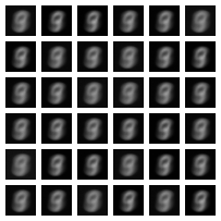
Finally, let me share an implementation of WGAN-GP, using MNIST as the dataset—readers are welcome to modify it and play around~
https://github.com/bojone/gan/
Training progress display~
 0
0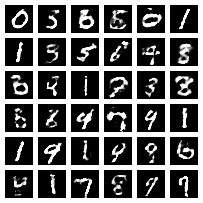 100
100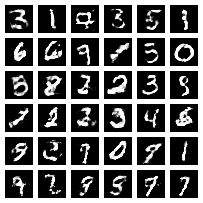 200
200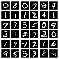 300
300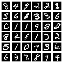 400
400
Translated automatically with claude-sonnet-5; all equations are reproduced verbatim from the source. Copyright remains with the original author.