From Wasserstein Distance and Duality Theory to WGAN
 Which bulldozer company is the best? For lowest cost, go with Wasserstein
Back in 2017 I wrote a post called The Art of Mutual Sparring: Getting to WGAN-GP from Scratch, which introduced WGAN from a relatively accessible angle. In that piece, WGAN felt more like a result plucked out of thin air, with not much apparent connection to the Wasserstein distance.
In this post, we'll discuss WGAN from a more mathematical viewpoint. Of course, this post isn't purely about GANs — it focuses mainly on understanding the Wasserstein distance and its duality theory. It was inspired by the well-known English-language post Wasserstein GAN and the Kantorovich-Rubinstein Duality; the content here largely follows it, but I've trimmed some redundant parts and filled in places that felt insufficiently explained or a bit vague. Either way, let me first pay tribute to that predecessor and their article.
(Note: fully understanding this post requires some background in multivariable calculus, probability theory, and linear algebra. Also, this post really is long and does contain a lot of formulas — but it's genuinely not complicated or hard to follow, so don't be scared off by the equations.) more
The Wasserstein Distance
Obviously, the whole post will revolve around the Wasserstein distance (W-distance), and since the Wasserstein distance is defined in terms of the optimal transport cost, we need to first introduce that. Suppose we have two probability distributions $p(\boldsymbol{x}),q(\boldsymbol{x})$; then the optimal transport cost is defined as
\begin{equation}\mathcal{C}[p,q]=\inf_{\gamma\in \Pi[p,q]} \iint \gamma(\boldsymbol{x},\boldsymbol{y}) c(\boldsymbol{x},\boldsymbol{y}) d\boldsymbol{x}d\boldsymbol{y}\label{eq:ot}\end{equation}
In fact, this is arguably the single most central definition in optimal transport theory.
Trust me, equation $\eqref{eq:ot}$ isn't as scary as it looks. Let's go through it term by term.
The Cost Function
First, look at $c(\boldsymbol{x},\boldsymbol{y})$: it's a cost function representing the cost of transporting from $\boldsymbol{x}$ to $\boldsymbol{y}$. A common choice is some power of the Euclidean distance:
\begin{equation}c(\boldsymbol{x},\boldsymbol{y}) = \Vert\boldsymbol{x}-\boldsymbol{y}\Vert^{\rho}\end{equation}
We then write
\begin{equation}\mathcal{W}_{\rho}[p,q]=\left(\mathcal{C}[p,q]\right)^{1/\rho}\end{equation}
and $\mathcal{W}_{\rho}[p,q]$ is what's called the "Wasserstein distance" (more precisely, the "Wasserstein-$\rho$ distance"). As you can see, the optimal transport cost $\mathcal{C}[p,q]$ is a more general notion than the Wasserstein distance $\mathcal{W}_{\rho}[p,q]$, so in what follows we'll mainly work with $\mathcal{C}[p,q]$. When $\rho=1$, the optimal transport cost coincides with the corresponding Wasserstein distance.
In general, the Euclidean distance $\Vert\boldsymbol{x}-\boldsymbol{y}\Vert$ could be replaced by a more general distance, but the specific choice isn't especially important, because many norms are equivalent to each other — and this norm-equivalence means that the W-distances one ends up defining turn out to be roughly comparable regardless of the choice.
Minimizing the Cost
Now let's look at $\gamma$. The condition $\gamma\in \Pi[p,q]$ means:
\begin{equation}\int \gamma(\boldsymbol{x},\boldsymbol{y}) d\boldsymbol{y}=p(\boldsymbol{x})\quad\text{and}\quad\int \gamma(\boldsymbol{x},\boldsymbol{y}) d\boldsymbol{x}=q(\boldsymbol{y})\end{equation}
In other words, $\gamma$ is a joint distribution whose marginals are exactly the original $p$ and $q$.
In fact, $\gamma$ describes a transport plan. Without loss of generality, let $p$ be the original distribution and $q$ be the target distribution. $p(\boldsymbol{x})$ means that there is originally a quantity $p(\boldsymbol{x})$ of goods at location $\boldsymbol{x}$, while $q(\boldsymbol{x})$ refers to the quantity of goods that should ultimately be stored at $\boldsymbol{x}$. If $p(\boldsymbol{x}) > q(\boldsymbol{x})$, then some of the goods at $\boldsymbol{x}$ need to be shipped elsewhere; conversely, if $p(\boldsymbol{x}) < q(\boldsymbol{x})$, then goods need to be shipped in from elsewhere to $\boldsymbol{x}$. And $\gamma(\boldsymbol{x}, \boldsymbol{y})$ means: move an amount $\gamma(\boldsymbol{x}, \boldsymbol{y})d\boldsymbol{x}$ of stuff from $\boldsymbol{x}$ to $\boldsymbol{y}$.
Finally there's $\inf$, which denotes the infimum — in simple terms, taking the minimum. That is, among all transport plans, we want to find the one whose total transport cost $\iint \gamma(\boldsymbol{x},\boldsymbol{y}) c(\boldsymbol{x},\boldsymbol{y}) d\boldsymbol{x}d\boldsymbol{y}$ is smallest; the cost of that plan is exactly the quantity $\mathcal{C}[p,q]$ we want to compute. If we replace "goods" in the analogy above with "earth," then the optimal transport cost is precisely the cost of the most efficient way to "move dirt" — which is why the Wasserstein distance is also often called the "Earth Mover's Distance."
Finally, let's adapt a picture from the English blog post mentioned above to illustrate this "earth-moving" process:
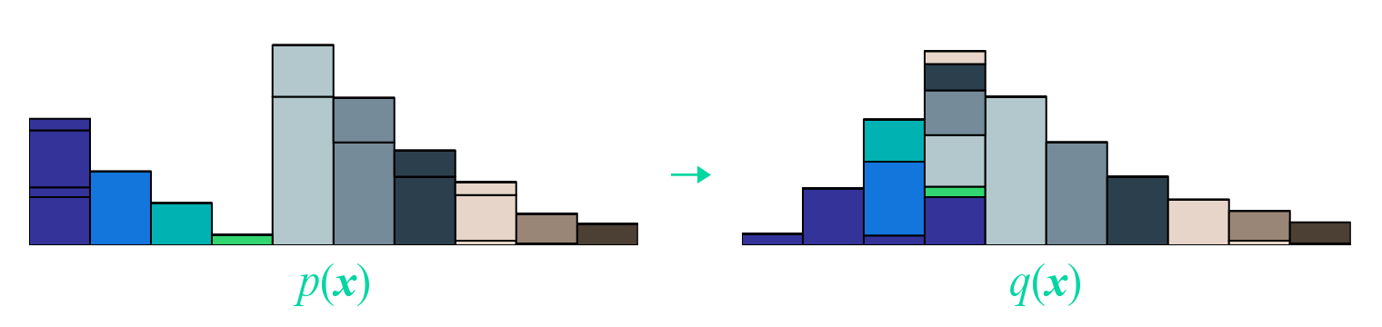 Illustration of the earth mover's distance. The dirt at each point of p(x) on the left is split into several parts and shipped to the same-colored positions in q(x) on the right (or left in place)
Matrix Form
Having gone through the meaning of each term, let's now restate the problem in full: what we're actually computing is the minimum of
\begin{equation}\iint \gamma(\boldsymbol{x},\boldsymbol{y}) c(\boldsymbol{x},\boldsymbol{y}) d\boldsymbol{x}d\boldsymbol{y}\label{eq:ot-t}\end{equation}
where $c(\boldsymbol{x},\boldsymbol{y})$ is given in advance, subject to the constraint that
\begin{equation}\int \gamma(\boldsymbol{x},\boldsymbol{y}) d\boldsymbol{y}=p(\boldsymbol{x}),\quad\int \gamma(\boldsymbol{x},\boldsymbol{y}) d\boldsymbol{x}=q(\boldsymbol{y}),\quad \gamma(\boldsymbol{x},\boldsymbol{y})\geq 0\label{eq:ot-c}\end{equation}
Staring closely at equation $\eqref{eq:ot-t}$, and keeping in mind that an integral is just a limiting form of a sum, we can discretize $\gamma(\boldsymbol{x},\boldsymbol{y})$ and $c(\boldsymbol{x},\boldsymbol{y})$ and treat them as very, very long (column) vectors $\boldsymbol{\Gamma}$ and $\boldsymbol{C}$:
\begin{equation}\boldsymbol{\Gamma}=\begin{pmatrix} \gamma(\boldsymbol{x}_1, \boldsymbol{y}_1) \\ \gamma(\boldsymbol{x}_1, \boldsymbol{y}_2) \\ \vdots \\ \hline \gamma(\boldsymbol{x}_2, \boldsymbol{y}_1) \\ \gamma(\boldsymbol{x}_2, \boldsymbol{y}_2) \\ \vdots \\ \hline \vdots \\ \hline \gamma(\boldsymbol{x}_n, \boldsymbol{y}_1) \\ \gamma(\boldsymbol{x}_n, \boldsymbol{y}_2) \\ \vdots \\ \hline \vdots \\ \end{pmatrix},\quad \boldsymbol{C}=\begin{pmatrix} c(\boldsymbol{x}_1, \boldsymbol{y}_1) \\ c(\boldsymbol{x}_1, \boldsymbol{y}_2) \\ \vdots \\ \hline c(\boldsymbol{x}_2, \boldsymbol{y}_1) \\ c(\boldsymbol{x}_2, \boldsymbol{y}_2) \\ \vdots \\ \hline \vdots \\ \hline c(\boldsymbol{x}_n, \boldsymbol{y}_1) \\ c(\boldsymbol{x}_n, \boldsymbol{y}_2) \\ \vdots \\ \hline \vdots \\ \end{pmatrix}\label{eq:lp-ot-t1}\end{equation}
So equation $\eqref{eq:ot-t}$ amounts to multiplying corresponding entries of $\boldsymbol{\Gamma}$ and $\boldsymbol{C}$ and summing them up — isn't that exactly the inner product $\langle\boldsymbol{\Gamma},\boldsymbol{C}\rangle$?
If that's not clear yet, stare a bit longer at equation $\eqref{eq:ot-t}$, picturing in your mind the process of discretizing $\boldsymbol{x},\boldsymbol{y}$ into small intervals, and recalling the definition of an integral; I believe it isn't too hard to see. Once you've grasped this, we can treat the constraint $\eqref{eq:ot-c}$ the same way: view $p(\boldsymbol{x}),q(\boldsymbol{x})$ as long vectors respectively, then stack them together and turn the integral into a sum as well. At that point the constraint $\eqref{eq:ot-c}$ can also be written in matrix form $\boldsymbol{A}\boldsymbol{\Gamma}=\boldsymbol{b}$:
\begin{equation}\underbrace{\left( \begin{array}{ccc|ccc|c|ccc|c} 1 & 1 & \dots & 0 & 0 & \dots & \dots & 0 & 0 & \dots & \dots \\ 0 & 0 & \dots & 1 & 1 & \dots & \dots & 0 & 0 & \dots & \dots \\ \vdots & \vdots & \ddots & \vdots & \vdots & \ddots & \ddots & \vdots & \vdots & \ddots & \ddots \\ 0 & 0 & \dots & 0 & 0 & \dots & \dots & 1 & 1 & \dots & \dots \\ \vdots & \vdots & \ddots & \vdots & \vdots & \ddots & \ddots & \vdots & \vdots & \ddots & \ddots \\ \hline 1 & 0 & \dots & 1 & 0 & \dots & \dots & 1 & 0 & \dots & \dots \\ 0 & 1 & \dots & 0 & 1 & \dots & \dots & 0 & 1 & \dots & \dots \\ \vdots & \vdots & \ddots & \vdots & \vdots & \ddots & \ddots & \vdots & \vdots & \ddots & \ddots \\ 0 & 0 & \dots & 0 & 0 & \dots & \dots & 0 & 0 & \dots & \dots \\ \vdots & \vdots & \ddots & \vdots & \vdots & \ddots & \ddots & \vdots & \vdots & \ddots & \ddots \\ \end{array} \right)}_{\Large\boldsymbol{A}}\,\, \underbrace{\begin{pmatrix} \gamma(\boldsymbol{x}_1, \boldsymbol{y}_1) \\ \gamma(\boldsymbol{x}_1, \boldsymbol{y}_2) \\ \vdots \\ \hline \gamma(\boldsymbol{x}_2, \boldsymbol{y}_1) \\ \gamma(\boldsymbol{x}_2, \boldsymbol{y}_2) \\ \vdots \\ \hline \vdots \\ \hline \gamma(\boldsymbol{x}_n, \boldsymbol{y}_1) \\ \gamma(\boldsymbol{x}_n, \boldsymbol{y}_2) \\ \vdots \\ \hline \vdots \\ \end{pmatrix}}_{\Large\boldsymbol{\Gamma}} \,\,=\,\, \underbrace{\begin{pmatrix} p(\boldsymbol{x}_1) \\ p(\boldsymbol{x}_2) \\ \vdots \\ p(\boldsymbol{x}_n) \\ \vdots \\ \hline q(\boldsymbol{y}_1) \\ q(\boldsymbol{y}_2) \\ \vdots \\ q(\boldsymbol{y}_n) \\ \vdots \\ \end{pmatrix}}_{\Large\boldsymbol{b}}\label{eq:lp-ot-t2}\end{equation}
Lastly, don't forget $\boldsymbol{\Gamma}\geq 0$, which says that every component of $\boldsymbol{\Gamma}$ is non-negative.
A Linear Programming Problem
The problem can now be described in one line:
\begin{equation}\min_{\boldsymbol{\Gamma}}\big\{\langle\boldsymbol{\Gamma},\boldsymbol{C}\rangle\,\big|\,\boldsymbol{A}\boldsymbol{\Gamma}=\boldsymbol{b},\,\boldsymbol{\Gamma}\geq 0\big\}\label{eq:lp-ot}\end{equation}
This is exactly the "minimize a linear function subject to linear constraints" problem — the linear programming problem we already encountered back in high school! So, although the original problem looked quite complicated, with its integrals and infima, after rewriting it, it's essentially a not-too-mysterious linear programming problem (though "not too mysterious" certainly doesn't mean "easy to solve").
Linear Programming and Duality
Let's rewrite the linear programming problem using more general notation. There are two common forms:
\begin{equation}\min_{\boldsymbol{x}}\big\{\boldsymbol{c}^{\top}\boldsymbol{x}\,\big|\,\boldsymbol{A}\boldsymbol{x}=\boldsymbol{b},\,\boldsymbol{x}\geq 0\big\}\quad\text{or}\quad \min_{\boldsymbol{x}}\big\{\boldsymbol{c}^{\top}\boldsymbol{x}\,\big|\,\boldsymbol{A}\boldsymbol{x}\geq \boldsymbol{b},\,\boldsymbol{x}\geq 0\big\}\end{equation}
These two forms are essentially equivalent, though the first is a bit simpler to discuss (really just a bit — there's no fundamental difference). From equation $\eqref{eq:lp-ot}$ we know that we're only concerned with the first form here.
Note that, to avoid confusion, we need to state the sizes of the various vectors involved. Assume every vector is a column vector, so that after transposition $^\top$ represents a row vector. $\boldsymbol{x},\boldsymbol{c}\in\mathbb{R}^n$ are both $n$-dimensional vectors, where $\boldsymbol{c}$ are the weights, and $\boldsymbol{c}^{\top}\boldsymbol{x}$ is the weighted sum over the components of $\boldsymbol{x}$; $\boldsymbol{b}\in\mathbb{R}^m$ is an $m$-dimensional vector, so naturally $\boldsymbol{A}\in\mathbb{R}^{m\times n}$ is an $m\times n$ matrix, and $\boldsymbol{A}\boldsymbol{x}=\boldsymbol{b}$ effectively describes $m$ equality constraints.
Weak Duality
In programming and optimization problems, "duality" is an extremely important concept. Roughly speaking, "duality" refers to some transformation that turns the original problem into an equivalent but seemingly very different new problem:
\begin{equation}\text{original problem}\quad\xrightarrow{\text{dual transform}}\quad \text{new problem}\end{equation}
The reason it's called "duality" is that applying the same kind of transformation to the new problem usually gets you back to the original problem:
\begin{equation}\text{new problem}\quad\xrightarrow{\text{dual transform}}\quad \text{original problem}\end{equation}
That is, "duality" is like a mirror: the original problem and the new problem are like an "object" and its "reflection." Solving one is equivalent to solving the other. So it just comes down to which of the two is easier.
You might wonder: how is "duality" different from equivalent reformulations in mathematics, such as the "contrapositive"? There's really no fundamental difference — both "duality" and "contrapositive" describe statements fully equivalent to the original. But "duality" tends to look very different from the original statement, whereas the "contrapositive" is merely a logical rearrangement of it. From a linear-algebra perspective, "duality" is analogous to the relationship between a subspace and its orthogonal complement.
Max vs. Min
Let's first introduce the "weak duality" form, whose derivation is fairly simple.
Our goal is $\min\limits_{\boldsymbol{x}}\big\{\boldsymbol{c}^{\top}\boldsymbol{x}\,\big|\,\boldsymbol{A}\boldsymbol{x}=\boldsymbol{b},\,\boldsymbol{x}\geq 0\big\}$; suppose the minimum is attained at $\boldsymbol{x}^*$, so we have $\boldsymbol{A}\boldsymbol{x}^*=\boldsymbol{b}$. We can multiply both sides by some $\boldsymbol{y}^{\top}\in\mathbb{R}^m$ to turn the equation into a scalar: $\boldsymbol{y}^{\top}\boldsymbol{A}\boldsymbol{x}^*=\boldsymbol{y}^{\top}\boldsymbol{b}$.
If we now assume $\boldsymbol{y}^{\top}\boldsymbol{A}\leq \boldsymbol{c}^{\top}$, then $\boldsymbol{y}^{\top}\boldsymbol{A}\boldsymbol{x}^*\leq \boldsymbol{c}^{\top}\boldsymbol{x}^*$ (since $\boldsymbol{x}^* \geq 0$), so $\boldsymbol{y}^{\top}\boldsymbol{b}\leq \boldsymbol{c}^{\top} \boldsymbol{x}^*$. In other words, under the condition $\boldsymbol{y}^{\top}\boldsymbol{A}\leq \boldsymbol{c}^{\top}$, any $\boldsymbol{y}^{\top}\boldsymbol{b}$ is always no greater than $\min\limits_{\boldsymbol{x}}\big\{\boldsymbol{c}^{\top}\boldsymbol{x}\,\big|\,\boldsymbol{A}\boldsymbol{x}=\boldsymbol{b},\,\boldsymbol{x}\geq 0\big\}$ — "always" meaning this holds even for the largest such value, so we get
\begin{equation}\max_{\boldsymbol{y}}\big\{\boldsymbol{b}^{\top}\boldsymbol{y}\,\big|\,\boldsymbol{A}^{\top}\boldsymbol{y}\leq \boldsymbol{c}\big\}\leq \min_{\boldsymbol{x}}\big\{\boldsymbol{c}^{\top}\boldsymbol{x}\,\big|\,\boldsymbol{A}\boldsymbol{x}=\boldsymbol{b},\,\boldsymbol{x}\geq 0\big\}\label{eq:weak-dual}\end{equation}
This is called the "weak duality" form; its shape is essentially: "the max of the left-hand side" is no bigger than "the min of the right-hand side."
A Few Remarks
Regarding weak duality, a few points may be worth clarifying:
1. We've now turned the original minimization problem into a maximization problem $\max\limits_{\boldsymbol{y}}\big\{\boldsymbol{b}^{\top}\boldsymbol{y}\,\big|\,\boldsymbol{A}^{\top}\boldsymbol{y}\leq \boldsymbol{c}\big\}$ — this already carries a flavor of duality. Of course, the reason this form of duality is called "weak" is that, at this point, we've only shown that this dual form is a lower bound on the original problem, not that the two are equal.
2. Weak duality holds for many optimization problems (including nonlinear ones). If the two sides are actually equal, then we have duality in the full sense, called strong duality.
3. In theory, to make further use of it we really do need to prove that the two sides of equation $\eqref{eq:weak-dual}$ are equal. But from a practical standpoint, the lower bound given by weak duality is often already good enough, since problems in deep learning are so complex that having even an approximate objective to optimize is already valuable.
4. You might ask: why did we assume $\boldsymbol{y}^{\top}\boldsymbol{A}\leq \boldsymbol{c}^{\top}$ instead of simply assuming $\boldsymbol{y}^{\top}\boldsymbol{A}=\boldsymbol{c}^{\top}$? The latter would certainly be much simpler, but the problem is that it's hard to achieve in practice, so we're stuck with the former assumption.
Strong Duality
As mentioned above, from a practical standpoint weak duality is already sufficient. But for readers interested in the complete theory, let's go ahead and work through "strong duality" too. Readers who only care about WGAN itself can feel free to skip this section.
Strong duality means
\begin{equation}\max_{\boldsymbol{y}}\big\{\boldsymbol{b}^{\top}\boldsymbol{y}\,\big|\,\boldsymbol{A}^{\top}\boldsymbol{y}\leq \boldsymbol{c}\big\} = \min_{\boldsymbol{x}}\big\{\boldsymbol{c}^{\top}\boldsymbol{x}\,\big|\,\boldsymbol{A}\boldsymbol{x}=\boldsymbol{b},\,\boldsymbol{x}\geq 0\big\}\label{eq:strong-dual}\end{equation}
Note that, as mentioned earlier, weak duality holds for many optimization problems, but strong duality does not always hold. For linear programming, however, strong duality does hold.
Farkas' Lemma
The proof of strong duality mainly relies on a result known as "Farkas' lemma":
For a fixed matrix $\boldsymbol{A}\in\mathbb{R}^{m\times n}$ and vector $\boldsymbol{b}\in\mathbb{R}^m$, exactly one of the following two statements holds:
1. There exists $\boldsymbol{x}\in \mathbb{R}^n$ with $\boldsymbol{x}\geq 0$ such that $\boldsymbol{A}\boldsymbol{x}=\boldsymbol{b}$;
2. There exists $\boldsymbol{y}\in \mathbb{R}^m$ such that $\boldsymbol{A}^{\top}\boldsymbol{y}\leq 0$ and $\boldsymbol{b}^{\top}\boldsymbol{y} > 0$.
What on earth does that mean? All these transposes, big and small — can someone explain this in plain language?
Actually, this lemma does have a fairly intuitive geometric interpretation, though translating that geometric picture into algebraic language isn't trivial. The starting point for the geometric interpretation is to consider the following set of vectors:
\begin{equation}\big\{\boldsymbol{A}\boldsymbol{x}\big|\boldsymbol{x}\in \mathbb{R}^n\text{and}\boldsymbol{x}\geq 0\big\}\end{equation}
The meaning of this set is: think of $\boldsymbol{A}$ as a combination of $n$ column vectors of dimension $m$,
\begin{equation}\boldsymbol{A}=(\boldsymbol{a}_1,\boldsymbol{a}_2,\dots,\boldsymbol{a}_n)\end{equation}
Then the set above is exactly all non-negative linear combinations of $\boldsymbol{a}_1,\boldsymbol{a}_2,\dots,\boldsymbol{a}_n$. What does such a set look like? The answer: it's a cone, as shown in the figure.
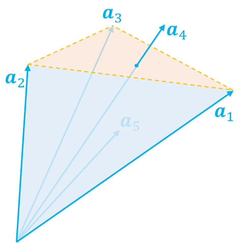 The non-negative linear combinations of given vectors form a cone bounded by those vectors
Now, given an arbitrary vector $\boldsymbol{b}$, there are obviously only two possibilities, and exactly one of them must hold: 1. it's inside the cone (including the boundary); 2. it's outside the cone. (This is of course a triviality, but once we translate it into algebraic language, it's no longer trivial.)
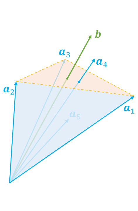 If the given vector lies inside the cone, it can be expressed as a non-negative linear combination
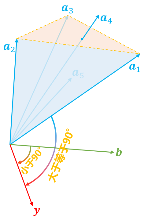 If the given vector lies outside the cone, we can find a "reference" vector to contrast it with
If it lies inside the cone, then by the very definition of a cone, it can be written as a non-negative linear combination of $\boldsymbol{a}_1,\boldsymbol{a}_2,\dots,\boldsymbol{a}_n$ (possibly in more than one way) — that is, there exists $\boldsymbol{x}\geq 0$ such that $\boldsymbol{A}\boldsymbol{x}=\boldsymbol{b}$, which is exactly the first case.
What if it's outside the cone? How do we express "outside the cone"? Of course we could just write down the negation of "inside the cone," but that wouldn't be very useful. If the vector $\boldsymbol{b}$ lies outside the cone, then we can always find a "reference" vector $\boldsymbol{y}$ that makes an angle of at least 90 degrees with every one of $\boldsymbol{a}_1,\boldsymbol{a}_2,\dots,\boldsymbol{a}_n$ — in vector terms, all the inner products are non-positive, i.e., $(\boldsymbol{a}_1^{\top}\boldsymbol{y}, \boldsymbol{a}_2^{\top}\boldsymbol{y}, \dots, \boldsymbol{a}_n^{\top}\boldsymbol{y}) \leq 0$, or written all at once as $\boldsymbol{A}^{\top}\boldsymbol{y} \leq 0$. Having found this "reference" vector, the angle between $\boldsymbol{b}$ and the reference must necessarily be less than 90 degrees, i.e., $\boldsymbol{b}^{\top}\boldsymbol{y} > 0$. Having one angle at least 90 degrees and the other less than 90 degrees guarantees that the vector $\boldsymbol{b}$ lies outside the cone formed by all the vectors. This is exactly the second case.
Of course, this doesn't amount to a rigorous proof — it's only a heuristic sketch; a rigorous proof would need to carefully justify why these non-negative linear combinations of vectors form a cone, which is beyond the scope of this post. The defining feature of Farkas' lemma is the "either-or": to prove statement 2 holds, it suffices to show statement 1 fails, and vice versa. This gives us a way to transform the problem.
From the Lemma to Strong Duality
With Farkas' lemma in hand, we can now prove strong duality. The idea of the proof is to show that $\max$ can be made arbitrarily close to $\min$.
As before, suppose the minimum of $\min$ is attained at $\boldsymbol{x}^*$, with minimum value $z^* = \boldsymbol{c}^{\top}\boldsymbol{x}^*$. Consider:
\begin{equation}\hat{\boldsymbol{A}} = \begin{pmatrix} \boldsymbol{A} \\ -\boldsymbol{c}^{\top} \end{pmatrix}, \quad \hat{\boldsymbol{b}}_{\epsilon} = \begin{pmatrix} \boldsymbol{b} \\ -z^* + \epsilon \end{pmatrix}, \quad \hat{\boldsymbol{y}} = \begin{pmatrix} \boldsymbol{y} \\ \alpha \end{pmatrix}\end{equation}
When $\epsilon > 0$, then for any $\boldsymbol{x} \geq 0$, $\hat{\boldsymbol{A}} \boldsymbol{x}$ can never equal $\hat{\boldsymbol{b}}_{\epsilon}$, because $\boldsymbol{c}^{\top} \boldsymbol{x}^* = z^*$ is already the minimum, so $-z^*$ is the largest value $-\boldsymbol{c}^{\top} \boldsymbol{x}$ can attain — it can't equal a strictly larger value $-z^* + \epsilon$.
Since we've just shown that case 1 fails, case 2 must hold: there exists $\hat{\boldsymbol{y}} = \begin{pmatrix} \boldsymbol{y} \\ \alpha \end{pmatrix}$ such that $\hat{\boldsymbol{A}}^{\top}\hat{\boldsymbol{y}}\leq 0$ and $\hat{\boldsymbol{b}}_{\epsilon}^{\top}\hat{\boldsymbol{y}} > 0$, which is equivalent to
\begin{equation}\boldsymbol{A}^{\top} \boldsymbol{y} \leq \alpha \boldsymbol{c}, \quad \boldsymbol{b}^{\top} \boldsymbol{y} > \alpha(z^* - \epsilon)\label{eq:whocare}\end{equation}
Next we show that $\alpha$ must be greater than 0. Since we already know $0 < \hat{\boldsymbol{b}}_{\epsilon}^{\top}\hat{\boldsymbol{y}} = \hat{\boldsymbol{b}}_{0}^{\top}\hat{\boldsymbol{y}} + \alpha\epsilon$, and $\hat{\boldsymbol{b}}_{0}^{\top}\hat{\boldsymbol{y}}$ has appeared here, let's also examine the case $\epsilon=0$: when $\epsilon = 0$, we have $\hat{\boldsymbol{A}} \boldsymbol{x}^* = \hat{\boldsymbol{b}}_0$, which satisfies the first case of Farkas' lemma, and therefore the second case cannot hold — and not satisfying the second case means "$\forall \hat{\boldsymbol{A}}^{\top}\hat{\boldsymbol{y}}\leq 0,\,\text{for all}\hat{\boldsymbol{b}}_{0}^{\top}\hat{\boldsymbol{y}}\leq 0$." But we've just shown $\hat{\boldsymbol{b}}_{0}^{\top}\hat{\boldsymbol{y}} + \alpha\epsilon > 0$, so we must have $\alpha > 0$.
Now that we know $\alpha > 0$, we can derive from equation $\eqref{eq:whocare}$ that
\begin{equation}\boldsymbol{A}^{\top} \big(\boldsymbol{y}/\alpha\big) \leq \boldsymbol{c}, \quad \boldsymbol{b}^{\top} \big(\boldsymbol{y}/\alpha\big) > z^* - \epsilon\end{equation}
which implies
\begin{equation}\max_{\boldsymbol{y}}\big\{\boldsymbol{b}^{\top}\boldsymbol{y}\,\big|\,\boldsymbol{A}^{\top}\boldsymbol{y}\leq \boldsymbol{c}\big\} > z^* - \epsilon\end{equation}
And weak duality already tells us that
\begin{equation}z^* \geq \max_{\boldsymbol{y}}\big\{\boldsymbol{b}^{\top}\boldsymbol{y}\,\big|\,\boldsymbol{A}^{\top}\boldsymbol{y}\leq \boldsymbol{c}\big\}\end{equation}
So $\max\limits_{\boldsymbol{y}}\big\{\boldsymbol{b}^{\top}\boldsymbol{y}\,\big|\,\boldsymbol{A}^{\top}\boldsymbol{y}\leq \boldsymbol{c}\big\}$ is sandwiched between $z^* - \epsilon$ and $z^*$, and since $\epsilon > 0$ is arbitrary, the two bounds can be made arbitrarily close, giving us
\begin{equation}\max_{\boldsymbol{y}}\big\{\boldsymbol{b}^{\top}\boldsymbol{y}\,\big|\,\boldsymbol{A}^{\top}\boldsymbol{y}\leq \boldsymbol{c}\big\}=z^*=\min_{\boldsymbol{x}}\big\{\boldsymbol{c}^{\top}\boldsymbol{x}\,\big|\,\boldsymbol{A}\boldsymbol{x}=\boldsymbol{b},\,\boldsymbol{x}\geq 0\big\}\end{equation}
which is precisely the strong duality result we set out to prove.
A Brief Remark
The proof of Farkas' lemma and strong duality may look somewhat roundabout, but it's actually one of the classic and important proofs in optimization theory. For beginners, it should come as quite a striking conceptual jolt. In our usual experience, transforming a statement is limited to "logical transformations," such as negations and contrapositives. But dual forms and Farkas' lemma give us results that "look completely different, yet happen to be equivalent."
Farkas' lemma and strong duality can also be extended to general convex optimization problems, following a similar proof strategy — though the discussion of regions and inequalities becomes more delicate and complex than in the linear programming case above. That said, I'm not a specialist in this area of optimization, so my understanding is only a rough one, and I won't pretend to expertise I don't have.
Wasserstein GAN
All right, with all that groundwork laid, we can finally derive the Wasserstein GAN — which, from the perspective of this post, turns out to be just a byproduct of the linear-programming dual form of the optimal transport cost.
The Dual of the Transport Cost
Before diving in, let's recap the thread of this post: we introduced the definition of the optimal transport cost $\eqref{eq:ot}$ on which the W-distance is based; then, through analysis, we found that it's actually a continuous version of an ordinary linear programming problem, via the transformations $\eqref{eq:lp-ot-t1},\eqref{eq:lp-ot-t2}$ and $\eqref{eq:lp-ot}$. So we spent a good chunk of the post learning about linear programming and its dual forms, eventually arriving at the conclusion $\eqref{eq:strong-dual}$.
What we need to do now is run this whole process in reverse: find the continuous-version counterpart of $\eqref{eq:strong-dual}$, i.e., find a dual expression for the optimal transport cost.
This turns out not to be too complicated either. From the conclusion $\eqref{eq:strong-dual}$ and equation $\eqref{eq:lp-ot}$, we get
\begin{equation}\min_{\boldsymbol{\Gamma}}\big\{\langle\boldsymbol{\Gamma},\boldsymbol{C}\rangle\,\big|\,\boldsymbol{A}\boldsymbol{\Gamma}=\boldsymbol{b},\,\boldsymbol{\Gamma}\geq 0\big\}=\max_{\boldsymbol{F}}\big\{\langle\boldsymbol{b},\boldsymbol{F}\rangle\,\big|\,\boldsymbol{A}^{\top}\boldsymbol{F}\leq \boldsymbol{C}\big\}\end{equation}
Note that in equation $\eqref{eq:lp-ot-t2}$, $\boldsymbol{b}$ is made up of two parts stitched together, so we can similarly write $\boldsymbol{F}$ as:
\begin{equation}\boldsymbol{F}=\begin{pmatrix} f(\boldsymbol{x}_1) \\ f(\boldsymbol{x}_2) \\ \vdots \\ f(\boldsymbol{x}_n) \\ \vdots \\ \hline g(\boldsymbol{y}_1) \\ g(\boldsymbol{y}_2) \\ \vdots \\ g(\boldsymbol{y}_n) \\ \vdots \\ \end{pmatrix}\end{equation}
Now $\langle\boldsymbol{b},\boldsymbol{F}\rangle$ can be written as
\begin{equation}\langle\boldsymbol{b},\boldsymbol{F}\rangle=\sum_n p(\boldsymbol{x}_n) f(\boldsymbol{x}_n) + \sum_n q(\boldsymbol{x}_n) g(\boldsymbol{x}_n)\end{equation}
or, in the corresponding integral form,
\begin{equation}\langle\boldsymbol{b},\boldsymbol{F}\rangle=\int \big[p(\boldsymbol{x}) f(\boldsymbol{x}) + q(\boldsymbol{x}) g(\boldsymbol{x})\big]d\boldsymbol{x}\end{equation}
Don't forget the constraint $\boldsymbol{A}^{\top}\boldsymbol{F}\leq \boldsymbol{C}$:
\begin{equation}\underbrace{\left( \begin{array}{ccccc|ccccc} 1 & 0 & \dots & 0 & \dots & 1 & 0 & \dots & 0 & \dots \\ 1 & 0 & \dots & 0 & \dots & 0 & 1 & \dots & 0 & \dots \\ \vdots & \vdots & \ddots & \vdots & \ddots & \vdots & \vdots & \ddots & \vdots & \ddots \\ \hline 0 & 1 & \dots & 0 & \dots & 1 & 0 & \dots & 0 & \dots \\ 0 & 1 & \dots & 0 & \dots & 0 & 1 & \dots & 0 & \dots \\ \vdots & \vdots & \ddots & \vdots & \ddots & \vdots & \vdots & \ddots & \vdots & \ddots \\ \hline \vdots & \vdots & \ddots & \vdots & \ddots & \vdots & \vdots & \ddots & \vdots & \ddots \\ \hline 0 & 0 & \dots & 1 & \dots & 1 & 0 & \dots & 0 & \dots \\ 0 & 0 & \ddots & 1 & \ddots & 0 & 1 & \ddots & 0 & \ddots \\ \vdots & \vdots & \ddots & \vdots & \ddots & \vdots & \vdots & \ddots & \vdots & \ddots \\ \hline \vdots & \vdots & \ddots & \vdots & \ddots & \vdots & \vdots & \ddots & \vdots & \ddots \\ \end{array} \right)}_{\Large\boldsymbol{A}^{\top}}\,\,\underbrace{\begin{pmatrix} f(\boldsymbol{x}_1) \\ f(\boldsymbol{x}_2) \\ \vdots \\ f(\boldsymbol{x}_n) \\ \vdots \\ \hline g(\boldsymbol{y}_1) \\ g(\boldsymbol{y}_2) \\ \vdots \\ g(\boldsymbol{y}_n) \\ \vdots \\ \end{pmatrix}}_{\Large\boldsymbol{F}}\,\,\leq\,\,\underbrace{\begin{pmatrix} c(\boldsymbol{x}_1, \boldsymbol{y}_1) \\ c(\boldsymbol{x}_1, \boldsymbol{y}_2) \\ \vdots \\ \hline c(\boldsymbol{x}_2, \boldsymbol{y}_1) \\ c(\boldsymbol{x}_2, \boldsymbol{y}_2) \\ \vdots \\ \hline \vdots \\ \hline c(\boldsymbol{x}_n, \boldsymbol{y}_1) \\ c(\boldsymbol{x}_n, \boldsymbol{y}_2) \\ \vdots \\ \hline \vdots \\ \end{pmatrix}}_{\Large \boldsymbol{C}}\end{equation}
Substituting this in, we find that this huge matrix computation is actually just saying the following:
\begin{equation}\forall i,j,\,\,f(\boldsymbol{x}_i) + g(\boldsymbol{y}_j)\leq c(\boldsymbol{x}_i,\boldsymbol{y}_j)\end{equation}
or, written directly,
\begin{equation}\forall \boldsymbol{x},\boldsymbol{y},\,\,f(\boldsymbol{x}) + g(\boldsymbol{y})\leq c(\boldsymbol{x},\boldsymbol{y})\end{equation}
From Duality to WGAN
We're finally nearing the end. We now have a dual form for the optimal transport cost $\eqref{eq:ot}$:
\begin{equation}\mathcal{C}[p,q]=\max_{f,g}\Bigg\{\int \big[p(\boldsymbol{x}) f(\boldsymbol{x}) + q(\boldsymbol{x}) g(\boldsymbol{x})\big]d\boldsymbol{x} \,\Bigg|\,\, f(\boldsymbol{x}) + g(\boldsymbol{y})\leq c(\boldsymbol{x},\boldsymbol{y})\Bigg\}\end{equation}
Note that from $f(\boldsymbol{x}) + g(\boldsymbol{y})\leq c(\boldsymbol{x},\boldsymbol{y})$ we get
\begin{equation}f(\boldsymbol{x}) + g(\boldsymbol{x})\leq c(\boldsymbol{x},\boldsymbol{x})=0\end{equation}
i.e., $g(\boldsymbol{x}) \leq - f(\boldsymbol{x})$, so we have
\begin{equation}\begin{aligned}p(\boldsymbol{x}) f(\boldsymbol{x}) + q(\boldsymbol{x}) g(\boldsymbol{x})&\leq p(\boldsymbol{x}) f(\boldsymbol{x}) + q(\boldsymbol{x}) [-f(\boldsymbol{x})]\\ & = p(\boldsymbol{x}) f(\boldsymbol{x}) - q(\boldsymbol{x}) f(\boldsymbol{x})\end{aligned}\end{equation}
This seems to suggest a conclusion: if $g = -f$, its maximum can't be smaller than the original maximum. In fact, this conclusion isn't entirely correct unless we require $c(\boldsymbol{x},\boldsymbol{y})$ to be a genuine distance (satisfying the triangle inequality) — for further discussion of this subtlety, see the comments section. Going forward, let's assume $c(\boldsymbol{x},\boldsymbol{y})$ is a distance function, which is exactly what WGAN assumes; in that case we can safely let $g=-f$, giving us
\begin{equation}\mathcal{C}[p,q]=\max_{f}\Bigg\{\int \big[p(\boldsymbol{x}) f(\boldsymbol{x}) - q(\boldsymbol{x}) f(\boldsymbol{x})\big]d\boldsymbol{x} \,\Bigg|\,\, f(\boldsymbol{x}) - f(\boldsymbol{y})\leq c(\boldsymbol{x},\boldsymbol{y})\Bigg\}\label{eq:ot-dual-u}\end{equation}
This is the dual form of the optimal transport cost $\eqref{eq:ot}$ that we've been after. In particular, when $c(\boldsymbol{x},\boldsymbol{y}) = \Vert \boldsymbol{x}-\boldsymbol{y}\Vert$, we have $\mathcal{C}[p,q] = \mathcal{W}_1[p,q]$, i.e.,
\begin{equation}\mathcal{W}_1[p,q]=\max_{f}\Bigg\{\int \big[p(\boldsymbol{x}) f(\boldsymbol{x}) - q(\boldsymbol{x}) f(\boldsymbol{x})\big]d\boldsymbol{x} \,\Bigg|\,\, f(\boldsymbol{x}) - f(\boldsymbol{y})\leq \Vert \boldsymbol{x}-\boldsymbol{y}\Vert\Bigg\}\label{eq:wd-dual-u}\end{equation}
This is exactly the W-distance that WGAN uses, where the constraint is usually written as $\Vert f\Vert_{L}\leq 1$, known as the Lipschitz constraint. From this derivation, we can also see that, in theory, the $c(\boldsymbol{x},\boldsymbol{y})$ in WGAN could be any more general distance function, not necessarily the Euclidean distance — but since many distances are equivalent to each other, and the distance here only serves to impose a constraint on the discriminator, choosing the Euclidean distance is simply good enough in practice.
Since $p,q$ are both probability distributions, we can write this in sampling form:
\begin{equation}\mathcal{W}_1[p,q]=\max_{f,\,\Vert f\Vert_{L}\leq 1}\mathbb{E}_{\boldsymbol{x}\sim p(\boldsymbol{x})}[f(\boldsymbol{x})] - \mathbb{E}_{\boldsymbol{x}\sim q(\boldsymbol{x})}[f(\boldsymbol{x})]\end{equation}
This is the loss used for WGAN's discriminator, and naturally, the whole WGAN training process is
\begin{equation}\min_{G}\max_{f,\,\Vert f\Vert_{L}\leq 1}\mathbb{E}_{\boldsymbol{x}\sim p(\boldsymbol{x})}[f(\boldsymbol{x})] - \mathbb{E}_{\boldsymbol{z}\sim q(\boldsymbol{z})}[f(G(\boldsymbol{z}))]\end{equation}
And so, the long-awaited WGAN has finally made its appearance. All that's left is the question of how to impose the Lipschitz constraint — see The Lipschitz Constraint in Deep Learning: Generalization and Generative Models for more on that.
Finally Done Writing
This post mainly introduced the optimal transport cost and the Wasserstein distance, showed how it can be turned into a linear programming problem, went on to introduce the duality theory of linear programming, and finally derived the dual form of the Wasserstein distance — which can be used to train generative models, i.e., WGAN and the series of extensions that followed it.
This post is a simple write-up of what I learned while studying linear programming and its duality theory, and it should be of some value to readers who are comfortable with linear algebra and want to understand WGAN at a more theoretical level. If anything here is unclear or you have criticisms, feel free to leave a comment.
Translated automatically with claude-sonnet-5; all equations are reproduced verbatim from the source. Copyright remains with the original author.