Diffusion Models from Scratch (31): Predict the Data, Not the Noise

生成扩散模型漫谈（三十一）：预测数据而非噪声 苏剑林 · 2025-11-24 · Machine Learning loss function generative model diffusion manifold

To this day, LDM (Latent Diffusion Models) remains the mainstream paradigm for diffusion models. By using an Encoder to heavily compress raw images, LDM can significantly reduce the computational cost of both training and inference, while also lowering the difficulty of the generation task itself — a genuine win-win. However, heavy compression also means information loss, and the "compress, generate, decompress" pipeline lacks some of the elegance of an end-to-end approach. As a result, there has always been a segment of the community that insists on "going back to pixel space," hoping to make diffusion models generate directly on raw data.

The work introduced in this post, Back to Basics: Let Denoising Generative Models Denoise, is a new contribution along exactly this line of thinking. Building on the fact that raw data typically lies on a low-dimensional submanifold, it proposes that the model should predict the data rather than the noise, giving rise to "JiT" (Just image Transformers), which significantly simplifies the architecture of pixel-space diffusion models.

Signal-to-Noise Ratio

There's no denying that today's "main force" in diffusion models is still LDM. Even the recently much-discussed RAE only claims that LDM's Encoder has become "outdated" and should be replaced with a newer, stronger one — it does not overturn the "compress first, then generate" paradigm. more

Part of the reason for this state of affairs, aside from LDM's ability to significantly reduce the computational cost of generating large images, is a key finding from researchers over a fairly long period: doing high-resolution diffusion generation directly in pixel space seems to come with some "inherent difficulties." Concretely, configurations that work well at low resolution (such as the noise schedule) tend to perform noticeably worse when applied to training high-resolution diffusion models — manifesting as slower convergence and worse FID than the low-resolution model.

Later, works such as Simple Diffusion identified the key reason behind this phenomenon: applying the same noise schedule to a higher-resolution image effectively increases the signal-to-noise ratio. Specifically, if we apply noise of the same intensity to a small image and a large image, then scale both to the same size, the large image will look noticeably cleaner. So when training a high-resolution diffusion model with the same noise schedule, the denoising task becomes implicitly easier, leading to problems like inefficient training and poor final performance.

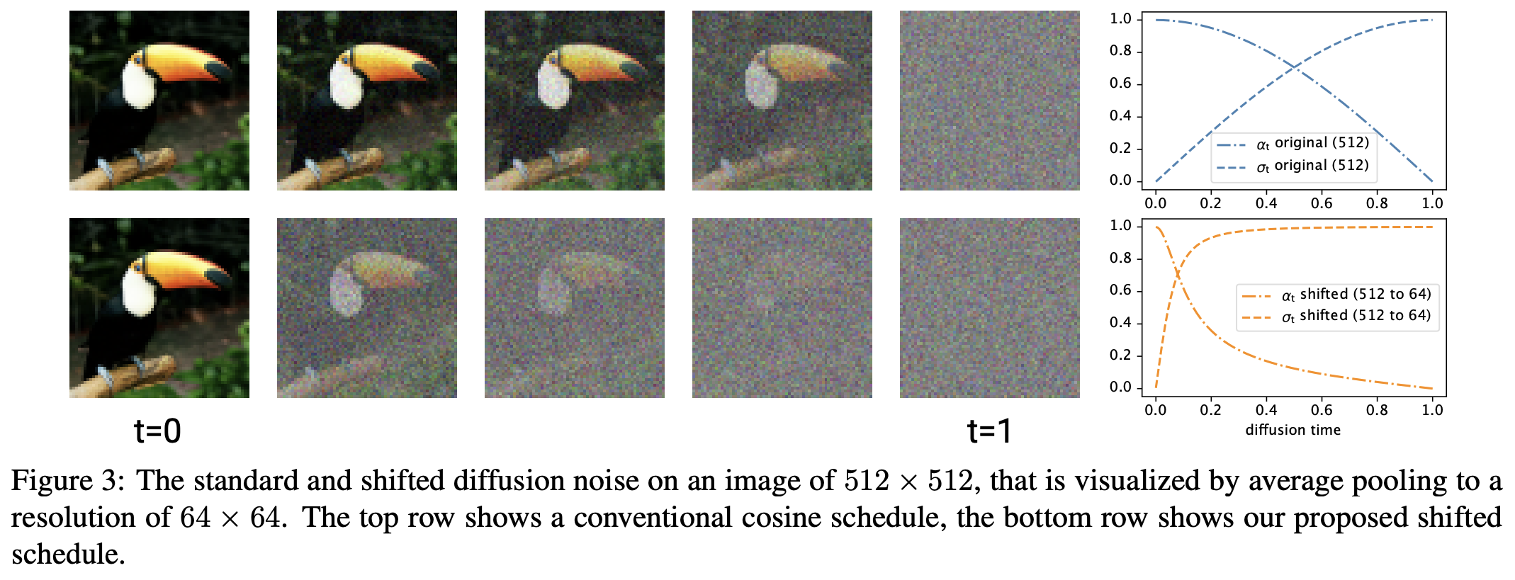Signal-to-noise ratio at different resolutions for the same noise

Once this cause is understood, the fix is not hard to figure out: adjust the noise schedule for the high-resolution diffusion model, increasing the noise intensity accordingly so that the signal-to-noise ratio is aligned at every step. For a more detailed discussion, see the earlier post Diffusion Models from Scratch (22): Signal-to-Noise Ratio and Large Image Generation (Part 1). Since then, pixel-space diffusion models have gradually caught up with LDM in terms of performance, and have begun to show their own competitiveness.

The Model Bottleneck

However, although pixel-space diffusion models have caught up with LDM on metrics like FID or IS, there remains another puzzling issue: to achieve metrics comparable to a low-resolution model, a high-resolution model must pay a much greater computational cost — more training steps, a bigger model, a larger feature map, and so on.

Some readers might think this is unremarkable: doesn't generating a bigger image naturally require more cost? At first glance that seems reasonable, but on closer thought it doesn't quite hold up. Large-image generation may indeed be intrinsically harder, but at least as far as metrics like FID/IS are concerned, it shouldn't be — because both metrics are computed after rescaling the generated results to a fixed size. This means that if we already have a batch of small images, it's trivially easy to obtain a batch of large images with unchanged FID/IS: just upsample each small image. This comes at essentially zero extra cost.

At this point someone might object, "but images obtained by upsampling lack detail!" — indeed, and that is exactly what was just described as "large-image generation being intrinsically harder," since it requires generating more detail. But the upsampling operation itself, at least in terms of FID and IS, is invariant. This implies that, in theory, given the same amount of compute, we should be able to obtain a large-image generative model with roughly the same FID/IS, even if it lacks detail. Yet this is not what happens in practice — often what we get instead is a model that is clearly worse across the board.

Let's make this concrete. Suppose our baseline is a small-image model of size $128\times 128$, which patchifies the input with patches of size $8\times 8$, linearly projects to 768 dimensions, feeds this into a ViT with hidden_size=768, and finally projects back to image size linearly. This configuration works well at resolution $128\times 128$. Now suppose we want to do large-image generation at $512\times 512$; all we need to do is change the patch size to $32\times 32$, and aside from a slight increase in the input/output projections, the overall computational cost is essentially unchanged.

The question now is: if we train a diffusion model at resolution $512\times 512$ using this model of roughly the same computational cost, can we get the same FID/IS as the $128\times 128$-resolution model?

Low-Dimensional Manifolds

For diffusion models predating JiT, the answer is: most likely not, because such a model exhibits a low-rank bottleneck at high resolution.

Diffusion models have had two mainstream paradigms so far: one predicting the noise, as in DDPM, and the other predicting the difference between the noise and the original image (the velocity), as in ReFlow. Both regression targets involve noise. Since the noise vector is sampled i.i.d. from a normal distribution, it "fills" the entire space — mathematically speaking, its support is the whole space. This means that in order for a model to successfully predict an arbitrary noise vector, it must, at the very least, avoid having a low-rank bottleneck; otherwise it couldn't even implement the identity map, let alone denoise.

Going back to the earlier example, once the patch size is changed to $32\times 32$, the input dimension becomes $32\times 32\times 3 = 3072$, which is then projected down to 768 dimensions — a naturally non-invertible operation. So if we still use this model to predict noise or velocity, it will perform poorly due to the low-rank bottleneck. The key issue here is that real models don't actually have unlimited fitting capacity; they inevitably have some fitting bottlenecks.

At this point, the core idea behind JiT should already be apparent:

Compared to noise, the raw data has a much lower effective dimensionality — that is, the raw data lies on a lower-dimensional submanifold. This means predicting the data is an "easier" task for the model than predicting the noise, and so the model should preferentially predict the raw data, especially when network capacity is limited.

In plain terms: raw data such as images generally has specific structure, so it's easier to predict, and hence the model should predict the image directly. This minimizes the impact of any low-rank bottleneck, and may even turn a disadvantage into an advantage.

Taken individually, none of these points is new: that noise has full support over the whole space, and that raw data typically lies on a low-dimensional manifold, are in some sense already "common knowledge"; nor is directly having the model predict the image rather than the noise a first attempt. But the most impressive thing about this paper is stringing all these points together into a coherent explanation — one that is both a genuine "aha" moment and yet, in hindsight, feels irrefutably like "it should have been this way all along."

Experimental Analysis

Of course, however reasonable it sounds, up to this point it's still just a conjecture, and the next step is to validate it experimentally. JiT contains many experiments, but the author believes the following three are the most worth highlighting.

First, we now have three candidate prediction targets: noise, velocity, and data, which can further be split into the model's prediction target and the loss function's regression target — giving nine possible combinations in total. Take ReFlow as an example: let $\boldsymbol{x}_0$ be the noise and $\boldsymbol{x}_1$ be the data. Its training objective is

\begin{equation}\mathbb{E}_{\boldsymbol{x}_0\sim p_0(\boldsymbol{x}_0),\boldsymbol{x}_1\sim p_1(\boldsymbol{x}_1)}\bigg[\bigg\Vert \boldsymbol{v}_{\boldsymbol{\theta}}\big(\underbrace{(\boldsymbol{x}_1 - \boldsymbol{x}_0)t + \boldsymbol{x}_0}_{\boldsymbol{x}_t}, t\big) - (\boldsymbol{x}_1 - \boldsymbol{x}_0)\bigg\Vert^2\bigg]\end{equation}

where $\boldsymbol{v}=\boldsymbol{x}_1 - \boldsymbol{x}_0$ is the velocity, so this is a loss whose regression target is velocity ($\boldsymbol{v}\text{-loss}$). If we model $\boldsymbol{v}_{\boldsymbol{\theta}}(\boldsymbol{x}_t, t)$ with a neural network, then the model's prediction target is also velocity ($\boldsymbol{v}\text{-pred}$). If, based on $\boldsymbol{x}_1 - \boldsymbol{x}_0=\frac{\boldsymbol{x}_1 - \boldsymbol{x}_t}{1-t}$, we parameterize $\boldsymbol{v}_{\boldsymbol{\theta}}(\boldsymbol{x}_t, t)$ as $\frac{\text{NN}_{\boldsymbol{\theta}}(\boldsymbol{x}_t, t) - \boldsymbol{x}_t}{1-t}$, then the prediction target of $\text{NN}$ becomes the data $\boldsymbol{x}_1$ ($\boldsymbol{x}\text{-pred}$).

The results of these nine combinations, on ViT models with and without a low-rank bottleneck, are shown below on the left:

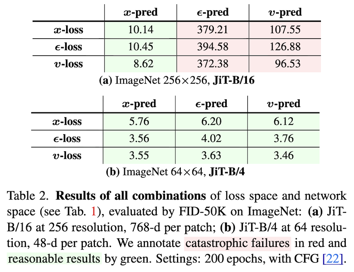Difference in performance across x/ε/v-pred/loss with and without a low-rank bottleneck 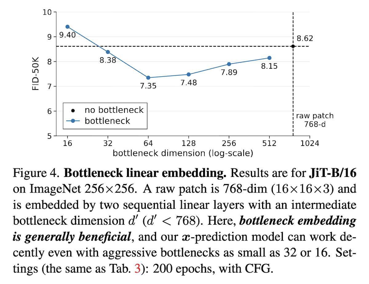Adding an appropriate low-rank bottleneck can actually help FID

We can see that without a low-rank bottleneck (b), the nine combinations don't differ much, but when the model does have a low-rank bottleneck (a), only the combination with data as the prediction target ($\boldsymbol{x}\text{-pred}$) manages to train successfully — the choice of regression target is secondary. This confirms the necessity of predicting data. In addition, the paper found that deliberately adding an appropriate low-rank bottleneck to JiT with $\boldsymbol{x}\text{-pred}$ actually improves FID, as shown in the figure on the right above.

Furthermore, the table below confirms that, by predicting the data, we can indeed obtain models at different resolutions with similar FID under similar compute and parameter budgets:

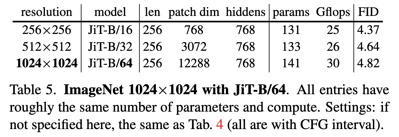Similar FID across different resolutions with similar compute and parameter counts

Finally, I also ran my own comparison, using a large-patch-size ViT model on CelebA HQ, comparing $\boldsymbol{x}\text{-pred}$ against $\boldsymbol{v}\text{-pred}$ as follows (trained fairly roughly, so just look at it comparatively):

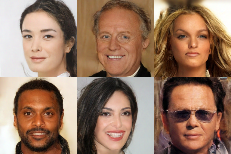Generation results predicting the original image 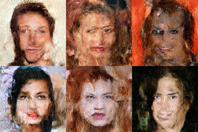Generation results predicting velocity

Further Thoughts

For more experimental results, readers are encouraged to check the original paper. In this section, let's discuss what changes JiT actually brings to diffusion models.

First, it does not set a new SOTA. Looking at the experimental tables in the paper, for the task of generating ImageNet images, it does not produce a new SOTA, but the gap from the best results is also small, so its performance can be considered SOTA-level, even if it doesn't clearly surpass it. On the other hand, if we take an already-SOTA non-$\boldsymbol{x}\text{-pred}$ model and convert it into a $\boldsymbol{x}\text{-pred}$ model, we probably wouldn't get significantly better results either.

That said, it may reduce the cost of achieving SOTA. Having the model predict data mitigates issues like the low-rank bottleneck, allowing us to revisit lightweight designs that were previously abandoned due to poor performance, or to "upgrade" a low-resolution SOTA model into a high-resolution one at relatively low additional training cost. From this perspective, the problem JiT truly solves is transferability from low resolution to high resolution.

Furthermore, JiT unifies the architectures used for visual understanding and generation. In fact, JiT is essentially the same ViT model used for visual understanding, and is quite similar to the GPT architecture used for text LLMs. This architectural unification makes it easier to design multimodal models that combine understanding and generation. By contrast, the standard architecture for earlier diffusion models was U-Net, which involves multiple levels of up/downsampling and multiple cross-scale skip connections, making the structure comparatively complex.

Seen this way, JiT can be said to have precisely identified the single most crucial skip connection within U-Net. Take the ReFlow example again: if we understand it in terms of modeling $\boldsymbol{v}_{\boldsymbol{\theta}}(\boldsymbol{x}_t, t)$, then in JiT we have $\boldsymbol{v}_{\boldsymbol{\theta}}(\boldsymbol{x}_t, t)=\frac{\text{NN}_{\boldsymbol{\theta}}(\boldsymbol{x}_t, t) - \boldsymbol{x}_t}{1-t}$, where the extra $-\boldsymbol{x}_t$ term is precisely a direct skip connection from input to output. U-Net, by contrast, doesn't bother figuring out which connection is critical — it simply adds such a skip connection to every up/downsampling block.

Finally, a brief digression. JiT also reminds the author of DDCM, which requires pre-sampling a huge matrix of "$T \times \text{img_size}$" as a codebook. The author once tried to approximate it using linear combinations of a finite number of random vectors, but failed — an experience that drove home just how thoroughly i.i.d. noise fills the entire space and resists compression. So upon reading JiT's claim that "data lies on a low-dimensional manifold, and predicting data is easier than predicting noise," the author found it almost instantly intuitive and convincing.

Summary

This post gave a brief introduction to JiT, which, based on the fact that raw data typically lies on a low-dimensional submanifold, proposes that models should preferentially predict data rather than noise/velocity. This reduces the modeling difficulty for diffusion models and lowers the likelihood of negative outcomes such as model collapse.