Diffusion Models Ramble (Part 22): Signal-to-Noise Ratio and Large-Image Generation (I)
If we take stock of the mainstream works on image diffusion models, we'll notice a pattern: most current work on high-resolution image generation (referred to below as "large-image generation") first transforms the image into a latent space via an Encoder (i.e., LDM, Latent Diffusion Model). Diffusion models trained directly in the raw pixel space, on the other hand, mostly operate at resolutions no higher than 6464 — and, conveniently, the Latent produced by LDM's AutoEncoder is also typically no larger than 6464. This naturally raises a series of questions: does diffusion modeling have some inherent difficulty with high-resolution generation? Can we directly generate high-resolution images in pixel space?
The paper Simple diffusion: End-to-end diffusion for high resolution images attempts to answer this question. It analyzes the difficulty of large-image generation through the lens of "signal-to-noise ratio," uses this analysis to optimize the noise schedule, and proposes techniques such as scaling up the architecture only at the lowest-resolution feature map and using multi-scale losses to preserve both training efficiency and quality. These modifications allowed the original paper to successfully train a pixel-space image diffusion model at resolutions up to 1024*1024. more
Revisiting LDM
Before getting into the main topic, let's first flip the question around: why has LDM managed to become the mainstream approach for diffusion models? In the author's view, there are mainly two reasons:
1. Whether in applications or in academic research, the main reason for using LDM is presumably efficiency: most current work directly reuses the pretrained AutoEncoder open-sourced by the LDM paper, whose Encoder maps a 512512 image down to a 6464 Latent. This means that, using only the compute and time budget of a 6464-resolution model, one can generate 512512 images — an obviously very appealing efficiency gain;
2. LDM happens to align well with the FID metric, which makes it look lossless: FID stands for "Fréchet Inception Distance," where "Inception" refers to using an ImageNet-pretrained InceptionV3 model as an encoder to encode images, after which the encoded features are assumed to follow a Gaussian distribution in order to compute the $\mathcal{W}$ distance. LDM also encodes images first via an Encoder, and although its Encoder is not identical to InceptionV3's, the two share some commonality. As a result, LDM tends to score as nearly lossless under FID.
Let's expand on this a bit further. LDM's AutoEncoder combines several components during training — its reconstruction loss isn't just the usual MAE or MSE, but also includes an adversarial loss and a perceptual loss. The adversarial loss ensures the sharpness of the reconstruction, while the perceptual loss ensures that the reconstruction is semantically and stylistically similar to the original. Perceptual Loss is quite similar to FID — both are similarity metrics computed from the features of an ImageNet-trained model, except that instead of InceptionV3 it uses VGG-16. Given the similarity of the two training tasks, one might guess that their feature spaces share a lot in common, so incorporating the Perceptual Loss indirectly ensures that FID degradation stays minimal.
Furthermore, LDM's Encoder performs dimensionality reduction on the raw image: for example, if the original image is 5125123, a naive patchify operation would yield 6464192, but LDM's Encoder instead outputs a feature map of size 64644 — a reduction to 1/48 of the naive size. To further reduce the variance of the encoded features and prevent the model from "memorizing by rote," LDM also applies an appropriate regularization term to the Encoder's output, either the KL-divergence term from VAE or the VQ regularization from VQ-VAE. Both the dimensionality reduction and the regularization compress the diversity of the features and improve their generalization ability, but they also make reconstruction harder, ultimately resulting in a lossy reconstruction.
At this point, the reason for LDM's success becomes "obvious": the combination of "dimensionality reduction + regularization" reduces the amount of information in the Latent, thereby reducing the difficulty of learning a diffusion model in the Latent space. Meanwhile, the presence of the Perceptual Loss ensures that although the reconstruction is lossy, the FID degradation is nearly negligible (in theory it would be even better if the Perceptual Loss's encoder used InceptionV3, matching FID exactly). As a result, from the perspective of the FID metric, LDM is essentially a free lunch — which is why both academia and industry are happy to adopt it.
The Signal-to-Noise Ratio
Although LDM is simple and efficient, it is, after all, lossy — its Latent can only preserve macroscopic semantics, while local details may be severely lost. In an earlier post, "Building Behind Closed Doors": A Brief Discussion of Multimodal Approaches (I): Lossless Input, the author expressed the view that when used as input, the best representation of an image is simply the raw pixel array. Based on this view, the author has recently been paying more attention to diffusion models trained directly in pixel space.
However, if we directly apply the diffusion model configuration used for low-resolution (e.g., 6464) images to high-resolution (e.g., 512512) large-image generation, we run into problems such as excessive compute cost and slow convergence, and the results also fall short of LDM (at least in terms of FID). Simple diffusion analyzes these problems one by one and proposes corresponding solutions. Among these, the author finds the use of the concept of "signal-to-noise ratio (SNR)" to analyze the low learning efficiency of high-resolution diffusion models to be the most illuminating part.
Specifically, Simple diffusion observes that if we add noise of a certain variance to a high-resolution image, its signal-to-noise ratio ends up being higher than that of a low-resolution image with the same noise variance added. Figure 3 of the original paper illustrates this very intuitively, as shown below. In the first row, a 512512 image has noise of a specific variance added, and is then downsampled (via average pooling) to 6464; in the second row, the same noise variance is added directly to the 64*64 image. It's clear that the first row's images are much clearer — i.e., they have a relatively higher signal-to-noise ratio.
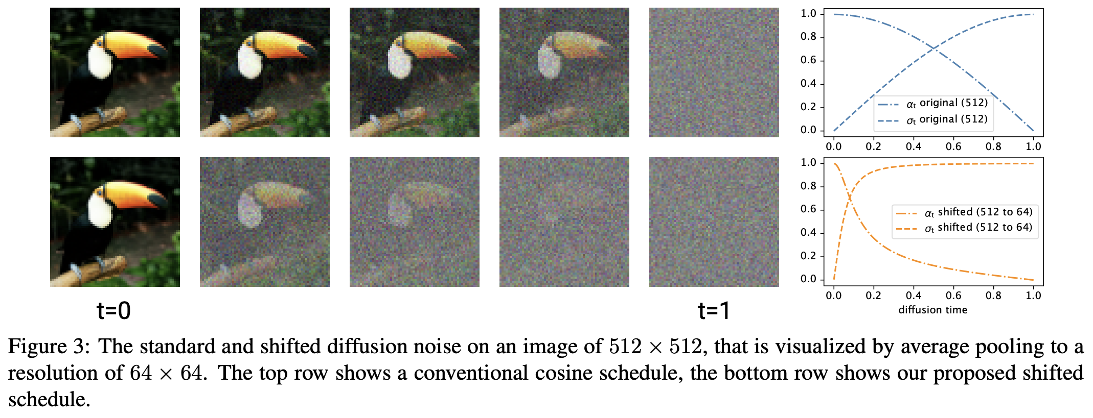 Signal-to-noise ratio at different resolutions with the same noise
As the name suggests, "signal-to-noise ratio" refers to the ratio between the strength of the signal and the strength of the noise. A higher signal-to-noise ratio (i.e., a lower proportion of noise) means denoising is easier — in other words, during training the Denoiser is mostly facing easy samples. But in reality, the difficulty of large-image generation is clearly higher, meaning our target is a harder model, yet we're feeding it easier samples — hence the resulting inefficiency in learning. A similar conclusion also appears in the contemporaneous work On the Importance of Noise Scheduling for Diffusion Models.
Aligning with the Low Resolution
We can also describe this mathematically. Following the notation used throughout this series, the process of constructing $\boldsymbol{x}_t$ via noise injection can be expressed as
\begin{equation}\boldsymbol{x}_t = \bar{\alpha}_t \boldsymbol{x}_0 + \bar{\beta}_t \boldsymbol{\varepsilon},\quad \boldsymbol{\varepsilon}\sim\mathcal{N}(\boldsymbol{0},\boldsymbol{I})\end{equation}
where $\bar{\alpha}_t,\bar{\beta}_t$ is what's called the Noise Schedule, satisfying $\bar{\alpha}_0=\bar{\beta}_T=1, \bar{\alpha}_T=\bar{\beta}_0=0$. In addition, there is generally an extra constraint — in DDPM, for instance, it is typically $\bar{\alpha}_t^2 + \bar{\beta}_t^2=1$, and we will adopt this constraint throughout this post.
For a random variable, the signal-to-noise ratio is the ratio of the squared mean to the variance. Given $\boldsymbol{x}_0$, the mean of $\boldsymbol{x}_t$ is clearly $\bar{\alpha}_t \mathbb{E}[\boldsymbol{x}_0]$, and the variance is $\bar{\beta}_t^2$, so the signal-to-noise ratio is $\frac{\bar{\alpha}_t^2}{\bar{\beta}_t^2}\mathbb{E}[\boldsymbol{x}_0]^2$. Since we are always discussing this conditioned on $\boldsymbol{x}_0$, we can simply say that the signal-to-noise ratio is $SNR(t) = \frac{\bar{\alpha}_t^2}{\bar{\beta}_t^2}$.
When we apply average pooling of size $s\times s$ to $\boldsymbol{x}_t$, each $s\times s$ patch is reduced to a scalar by averaging, i.e.
\begin{equation}\frac{1}{s^2}\sum_{i=1}^s \sum_{j=1}^s\boldsymbol{x}_t^{(i,j)} = \bar{\alpha}_t\left(\frac{1}{s^2}\sum_{i=1}^s \sum_{j=1}^s \boldsymbol{x}_0^{(i,j)}\right) + \bar{\beta}_t\left(\frac{1}{s^2}\sum_{i=1}^s \sum_{j=1}^s \boldsymbol{\varepsilon}^{(i,j)}\right) ,\quad \boldsymbol{\varepsilon}^{(i,j)}\sim\mathcal{N}(0, 1)\end{equation}
Average pooling doesn't change the mean, but it does reduce the variance, thereby increasing the signal-to-noise ratio — this follows from the additivity property of the normal distribution:
\begin{equation}\frac{1}{s^2}\sum_{i=1}^s \sum_{j=1}^s \boldsymbol{\varepsilon}^{(i,j)}\sim\mathcal{N}(0, 1/s^2)\end{equation}
Therefore, under the same Noise Schedule, if we downsample a high-resolution image via average pooling to match a low-resolution image, we find that the signal-to-noise ratio is higher — specifically, $s^2$ times higher than the original:
\begin{equation}SNR^{w\times h\to w/s\times h/s}(t) = SNR^{w/s\times h/s}(t) \times s^2 \end{equation}
Turning this around: if we already have a Noise Schedule $\bar{\alpha}_t^{w/s\times h/s},\bar{\beta}_t^{w/s\times h/s}$ tuned on low-resolution images, then when we want to scale up to a higher resolution, we should adjust the Noise Schedule to $\bar{\alpha}_t^{w\times h},\bar{\beta}_t^{w\times h}$ such that, after downsampling to the low resolution, its signal-to-noise ratio matches that of the already-tuned low-resolution Noise Schedule. This way, we can "inherit" as much as possible the learning efficiency of the existing low-resolution diffusion model, i.e.
\begin{equation} \frac{(\bar{\alpha}_t^{w\times h})^2}{(\bar{\beta}_t^{w\times h})^2} \times s^2 = \frac{(\bar{\alpha}_t^{w/s\times h/s})^2}{(\bar{\beta}_t^{w/s\times h/s})^2} \end{equation}
If we add the constraint $\bar{\alpha}_t^2 + \bar{\beta}_t^2=1$, then $\bar{\alpha}_t^{w\times h},\bar{\beta}_t^{w\times h}$ can be solved uniquely from $\bar{\alpha}_t^{w/s\times h/s},\bar{\beta}_t^{w/s\times h/s}$. This resolves the problem of setting the Noise Schedule for high-resolution diffusion.
Scaling Up the Architecture
To do a good job of diffusion generation for large images, besides adjusting the Noise Schedule, we also need to scale up the architecture — because as we've already said, large-image generation is a harder problem, and thus warrants a heavier-weight architecture.
The architectures commonly used in diffusion models are U-Net or U-ViT, both of which first progressively downsample and then progressively upsample. For example, given a 512512 input, we typically first run a block of computation, then downsample to 256256, run another block, downsample to 128128, and so on, down to some minimum resolution such as 1616. This process is then repeated in reverse — replacing downsampling with upsampling — until the resolution is restored to 512*512. By default, we distribute the parameters evenly across each block, but this means that the blocks near the input and output, which operate on very large inputs, end up with a sharply increased computational cost, leading to low training efficiency or even making training infeasible.
Simple diffusion proposes two countermeasures. First, it proposes downsampling right after the first layer (rather than the first block, since each block contains multiple layers), and going straight down to 128128 or even 6464 in one step; likewise, at the output end, upsampling happens only right before the last layer, going directly from 6464 or 128128 back up to 512512. This way, most of the model's blocks operate at a reduced resolution, lowering the overall compute cost. Second, it proposes that all the layers added when scaling up the model should be placed after the lowest resolution (i.e., 1616), rather than being spread evenly across blocks at every resolution — meaning the newly added layers all operate on 16*16 inputs, and even Dropout is only added to these low-resolution layers. This significantly reduces the compute burden that comes with increasing resolution.
In addition, to further stabilize training, the paper proposes a "multi-scale loss" training objective. By default, the loss of a diffusion model is equivalent to an MSE loss:
\begin{equation}\mathcal{L}=\frac{1}{wh}\Vert \boldsymbol{\varepsilon} - \boldsymbol{\epsilon}_{\boldsymbol{\theta}}(\bar{\alpha}_t \boldsymbol{x}_0 + \bar{\beta}_t \boldsymbol{\varepsilon}, t)\Vert^2\end{equation}
Simple diffusion generalizes this to
\begin{equation}\mathcal{L}_{s\times s} = \frac{1}{(w/s)(h/s)}\big\Vert \mathcal{D}_{w/s\times h/s}[\boldsymbol{\varepsilon}] - \mathcal{D}_{w/s\times h/s}[\boldsymbol{\epsilon}_{\boldsymbol{\theta}}(\bar{\alpha}_t \boldsymbol{x}_0 + \bar{\beta}_t \boldsymbol{\varepsilon}, t)]\big\Vert^2\end{equation}
where $\mathcal{D}_{w/s\times h/s}[\cdot]$ is a downsampling operator that transforms the input to $w/s\times h/s$ via average pooling. The original paper averages the losses over several choices of $s$ to obtain the final training objective. The purpose of this multi-scale loss is clear — much like adjusting the Noise Schedule via signal-to-noise-ratio alignment, it's meant to ensure that the trained high-resolution diffusion model is at least no worse than a model trained directly at low resolution.
As for the experiments, readers are encouraged to consult the original paper. The maximum resolution used in Simple diffusion's experiments is 1024*1024 (mentioned in the appendix), and the results are reasonably good. The ablation studies show that the techniques proposed above all yield improvements, and the final diffusion model trained directly in pixel space achieves results competitive with LDM.
Summary
In this post, we introduced Simple diffusion, a piece of work that explores how to train image diffusion models end-to-end directly in pixel space. It uses the concept of signal-to-noise ratio to explain the low training efficiency of high-resolution diffusion models, uses this analysis to guide the design of a new Noise Schedule, and explores how to scale up the model architecture while conserving compute cost as much as possible.
Translated automatically with claude-sonnet-5; all equations are reproduced verbatim from the source. Copyright remains with the original author.