Higher-Order MuP: A Simpler yet Smarter Spectral Condition Scaling
In the article An Initial Look at MuP: The Scaling Law for Hyperparameter Transfer Across Model Scales, we derived MuP (Maximal Update Parametrization) based on the scale invariance of forward propagation, backpropagation, loss increments, and feature changes. For some readers, this process may still have felt somewhat tedious, but in fact it was already noticeably simpler than the original paper. Keep in mind that we introduced MuP relatively completely within a single article, whereas the MuP paper is actually the fifth installment in the author's Tensor Programs series!
The good news, however, is that in a follow-up study, A Spectral Condition for Feature Learning, the author found a new way of understanding this (referred to below as the "spectral condition") that is more intuitive and concise than both the original MuP derivation and my own derivation, yet yields results even richer than MuP's. It can be seen as a higher-order version of MuP — a masterpiece that is simple without sacrificing sophistication.
Preliminaries
As the name suggests, the Spectral Condition is related to the Spectral Norm, and its starting point is a basic inequality about spectral norms:
\begin{equation}\Vert\boldsymbol{x}\boldsymbol{W}\Vert_2\leq \Vert\boldsymbol{x}\Vert_2 \Vert\boldsymbol{W}\Vert_2\label{neq:spec-2}\end{equation}more
Here $\boldsymbol{x}\in\mathbb{R}^{d_{in}}, \boldsymbol{W}\in\mathbb{R}^{d_{in}\times d_{out}}$, and as for $\Vert\cdot\Vert_2$, we can call it the "$2$ norm." For $\boldsymbol{x},\boldsymbol{x}\boldsymbol{W}$, which are vectors, the $2$ norm is simply the vector's magnitude; while $\boldsymbol{W}$ is a matrix, whose $2$ norm is also called the spectral norm — it equals the smallest constant $C$ such that $\Vert\boldsymbol{x}\boldsymbol{W}\Vert_2\leq C\Vert\boldsymbol{x}\Vert_2$ always holds. In other words, the above inequality is really just a direct corollary of the definition of the spectral norm, requiring no additional proof.
For more on the spectral norm, see the posts Lipschitz Constraints in Deep Learning: Generalization and Generative Models and The Road to Low-Rank Approximation (II): SVD; we won't elaborate further here. Matrices also have a simpler $F$ norm, which is a straightforward generalization of vector magnitude:
\begin{equation}\Vert \boldsymbol{W}\Vert_F = \sqrt{\sum_{i=1}^{d_{in}}\sum_{j=1}^{d_{out}}W_{i,j}^2}\end{equation}
From the perspective of singular values, the spectral norm equals the largest singular value of the matrix, while the $F$ norm equals the square root of the sum of squares of all the singular values. Similarly, we can define the "Nuclear Norm," which equals the sum of all singular values:
\begin{equation}\Vert \boldsymbol{W}\Vert_* = \sum_{i=1}^{\min(d_{in}, d_{out})} \sigma_i\end{equation}
Matrix norms like the spectral norm, the $F$ norm, and the nuclear norm — all of which can be expressed in terms of singular values — belong to the family of Schatten-p norms. Finally, let's define the RMS (Root Mean Square), which is a variant of vector magnitude:
\begin{equation}\Vert\boldsymbol{x}\Vert_{RMS} = \sqrt{\frac{1}{d_{in}}\sum_{i=1}^{d_{in}} x_i^2} = \frac{1}{\sqrt{d_{in}}}\Vert \boldsymbol{x}\Vert_2 \end{equation}
Generalizing this to matrices gives us $\Vert\boldsymbol{W}\Vert_{RMS} = \Vert \boldsymbol{W}\Vert_F/\sqrt{d_{in} d_{out}}$. This is actually easy to understand from the name: vector magnitude or the matrix $F$ norm can be called "Root Sum Square," while RMS replaces Sum with Mean, and it's mainly used as a measure of the average scale of the elements of a vector or matrix. Now substituting RMS into the inequality $\eqref{neq:spec-2}$, we obtain
\begin{equation}\Vert\boldsymbol{x}\boldsymbol{W}\Vert_{RMS}\leq \sqrt{\frac{d_{in}}{d_{out}}}\Vert\boldsymbol{x}\Vert_{RMS} \Vert\boldsymbol{W}\Vert_2\label{neq:spec-rms}\end{equation}
The Desired Properties
Our earlier approach to deriving MuP involved carefully analyzing the forms of forward propagation, backpropagation, loss increments, and feature change, and achieving their scale invariance by adjusting initialization and learning rate. After the spectral condition "distills the essence" of this, it turns out that just two points — forward propagation and feature change — are enough.
Simply put, the spectral condition requires that both the output and the increment of every layer be scale-invariant. What does this mean concretely? If we denote each layer simply as $\boldsymbol{x}_k= f(\boldsymbol{x}_{k-1}; \boldsymbol{W}_k)$, this statement can be translated as "we require every $\Vert\boldsymbol{x}_k\Vert_{RMS}$ and $\Vert\Delta\boldsymbol{x}_k\Vert_{RMS}$ to be $\Theta(1)$" (where $\Theta$ is the "Big Theta Notation"):
1. $\Vert\boldsymbol{x}_k\Vert_{RMS}=\Theta(1)$ is easy to understand — it represents the stability of forward propagation, and the previous article's derivation also included this requirement;
2. $\Delta\boldsymbol{x}_k$ represents the amount of change in $\boldsymbol{x}_k$ caused by the change in parameters, so $\Vert\Delta\boldsymbol{x}_k\Vert_{RMS}=\Theta(1)$ combines the requirements of backpropagation and feature change.
Some readers might wonder: shouldn't there also be at least a requirement on the "loss increment"? Actually, no. In fact, we can prove that if every layer's $\Vert\boldsymbol{x}_k\Vert_{RMS}$ and $\Vert\Delta\boldsymbol{x}_k\Vert_{RMS}$ are both $\Theta(1)$, then $\Delta\mathcal{L}$ is automatically $\Theta(1)$ as well. This is the first delightful aspect of the spectral condition idea: it reduces the four conditions originally needed to derive MuP down to two, cutting down the steps of analysis.
The proof isn't difficult. The key here is that we've assumed $\Vert\boldsymbol{x}_k\Vert_{RMS}=\Theta(1)$ and $\Vert\Delta\boldsymbol{x}_k\Vert_{RMS}=\Theta(1)$ hold for every layer, so naturally they also hold for the last layer. Suppose the model has $K$ layers in total, and the per-sample loss function is $\ell$; then it is a function of $\boldsymbol{x}_K$, i.e., $\ell(\boldsymbol{x}_K)$ — for simplicity we've omitted the label input here, since it isn't a variable for the analysis below.
By assumption, $\Vert\boldsymbol{x}_K\Vert_{RMS}$ is $\Theta(1)$, so $\ell(\boldsymbol{x}_K)$ is naturally $\Theta(1)$ as well; and since $\Vert\Delta\boldsymbol{x}_K\Vert_{RMS}$ is $\Theta(1)$, $\Vert\boldsymbol{x}_K + \Delta\boldsymbol{x}_K\Vert_{RMS}\leq \Vert\boldsymbol{x}_K\Vert_{RMS} + \Vert\Delta\boldsymbol{x}_K\Vert_{RMS}$ is also $\Theta(1)$, and hence $\ell(\boldsymbol{x}_K + \Delta\boldsymbol{x}_K)$ is $\Theta(1)$. Thus
\begin{equation}\Delta \ell = \ell(\boldsymbol{x}_K + \Delta\boldsymbol{x}_K) - \ell(\boldsymbol{x}_K) = \Theta(1)\end{equation}
So the per-sample loss increment $\Delta \ell$ is $\Theta(1)$, and since $\Delta\mathcal{L}$ is the average of all the $\Delta \ell$'s, it too is $\Theta(1)$. This proves that $\Vert\boldsymbol{x}_k\Vert_{RMS}=\Theta(1)$ and $\Vert\Delta\boldsymbol{x}_k\Vert_{RMS}=\Theta(1)$ automatically imply $\Delta\mathcal{L}=\Theta(1)$. The underlying reason is simply that $\Delta\mathcal{L}$ is a function of the output of the final layer and its increment — once both of those are stable, $\Delta\mathcal{L}$ is naturally stable too.
The Spectral Condition
Next, let's see how the two desired properties come about. Since neural networks are built primarily on matrix multiplications, let's first consider the simplest linear layer $\boldsymbol{x}_k = \boldsymbol{x}_{k-1} \boldsymbol{W}_k$, where $\boldsymbol{W}_k\in\mathbb{R}^{d_{k-1}\times d_k}$. To satisfy the condition $\Vert\boldsymbol{x}_k\Vert_{RMS}=\Theta(1)$, rather than assuming i.i.d. entries and then computing expectations and variances as in traditional initialization analysis, the spectral condition directly applies the inequality $\eqref{neq:spec-rms}$:
\begin{equation}\Vert\boldsymbol{x}_k\Vert_{RMS}\leq \sqrt{\frac{d_{k-1}}{d_k}}\Vert\boldsymbol{x}_{k-1}\Vert_{RMS}\, \Vert\boldsymbol{W}_k\Vert_2\end{equation}
Note that this inequality can achieve equality, and in a sense is the tightest possible bound — so if the input $\Vert\boldsymbol{x}_{k-1}\Vert_{RMS}$ already satisfies $\Theta(1)$, then in order to make the output satisfy $\Vert\boldsymbol{x}_k\Vert_{RMS}=\Theta(1)$, we need
\begin{equation}\sqrt{\frac{d_{k-1}}{d_k}}\Vert\boldsymbol{W}_k\Vert_2 = \Theta(1)\quad\Rightarrow\quad \Vert\boldsymbol{W}_k\Vert_2 = \Theta\left(\sqrt{\frac{d_k}{d_{k-1}}}\right)\label{eq:spec-c1}\end{equation}
This gives us the first spectral condition — a requirement on the spectral norm of $\boldsymbol{W}_k$. It has nothing to do with initialization or distributional assumptions; it's purely a consequence of analysis and algebra. This is, in my view, the second delightful aspect of the spectral condition — it simplifies the analytical process. Of course, we've omitted the basics of the spectral norm here; filling that in would likely make this section no shorter than an analysis under distributional assumptions, but distributional assumptions are ultimately more restrictive than this algebraic framework, which is more flexible.
Having analyzed $\Vert\boldsymbol{x}_k\Vert_{RMS}$, we now turn to $\Vert\Delta\boldsymbol{x}_k\Vert_{RMS}$. The increment $\Delta\boldsymbol{x}_k$ comes from two sources: first, the parameters change from $\boldsymbol{W}_k$ to $\boldsymbol{W}_k+\Delta \boldsymbol{W}_k$, and second, the change in parameters causes the input $\boldsymbol{x}_{k-1}$ to change from $\boldsymbol{x}_{k-1}$ to $\boldsymbol{x}_{k-1} + \Delta\boldsymbol{x}_{k-1}$. So
\begin{equation}\begin{aligned} \Delta\boldsymbol{x}_k =&\, (\boldsymbol{x}_{k-1} + \Delta\boldsymbol{x}_{k-1})(\boldsymbol{W}_k+\Delta \boldsymbol{W}_k) - \boldsymbol{x}_{k-1}\boldsymbol{W}_k \\[5pt] =&\, \boldsymbol{x}_{k-1} (\Delta \boldsymbol{W}_k) + (\Delta\boldsymbol{x}_{k-1})\boldsymbol{W}_k + (\Delta\boldsymbol{x}_{k-1})(\Delta \boldsymbol{W}_k) \end{aligned}\end{equation}
Hence
\begin{equation}\begin{aligned} \Vert\Delta\boldsymbol{x}_k\Vert_{RMS} =&\, \Vert\boldsymbol{x}_{k-1} (\Delta \boldsymbol{W}_k) + (\Delta\boldsymbol{x}_{k-1})\boldsymbol{W}_k + (\Delta\boldsymbol{x}_{k-1})(\Delta \boldsymbol{W}_k)\Vert_{RMS} \\[5pt] \leq&\, \Vert\boldsymbol{x}_{k-1} (\Delta \boldsymbol{W}_k)\Vert_{RMS} + \Vert(\Delta\boldsymbol{x}_{k-1})\boldsymbol{W}_k\Vert_{RMS} + \Vert(\Delta\boldsymbol{x}_{k-1})(\Delta \boldsymbol{W}_k)\Vert_{RMS} \\[5pt] \leq&\, \sqrt{\frac{d_{k-1}}{d_k}}\left({\begin{gathered}\Vert\boldsymbol{x}_{k-1}\Vert_{RMS}\,\Vert\Delta \boldsymbol{W}_k\Vert_2 + \Vert\Delta\boldsymbol{x}_{k-1}\Vert_{RMS}\,\Vert \boldsymbol{W}_k\Vert_2 \\[5pt] + \Vert\Delta\boldsymbol{x}_{k-1}\Vert_{RMS}\,\Vert\Delta \boldsymbol{W}_k\Vert_2\end{gathered}} \right) \end{aligned}\end{equation}
Analyzing this term by term:
\begin{equation}\underbrace{\Vert\boldsymbol{x}_{k-1}\Vert_{RMS}}_{\Theta(1)}\,\Vert\Delta \boldsymbol{W}_k\Vert_2 + \underbrace{\Vert\Delta\boldsymbol{x}_{k-1}\Vert_{RMS}}_{\Theta(1)}\,\underbrace{\Vert \boldsymbol{W}_k\Vert_2}_{\Theta\left(\sqrt{\frac{d_k}{d_{k-1}}}\right)} + \underbrace{\Vert\Delta\boldsymbol{x}_{k-1}\Vert_{RMS}}_{\Theta(1)}\,\Vert\Delta \boldsymbol{W}_k\Vert_2\end{equation}
From this we can see that to achieve $\Vert\Delta\boldsymbol{x}_k\Vert_{RMS}=\Theta(1)$, we need
\begin{equation}\Vert\Delta\boldsymbol{W}_k\Vert_2 = \Theta\left(\sqrt{\frac{d_k}{d_{k-1}}}\right)\label{eq:spec-c2}\end{equation}
This is the second spectral condition — a requirement on the spectral norm of $\Delta\boldsymbol{W}_k$.
The above analysis didn't take nonlinearity into account, but in fact, as long as the activation function is element-wise and its derivative is bounded by some constant (satisfied by common activations like ReLU, Sigmoid, and Tanh), the conclusion holds even when nonlinear activations are considered. This is exactly the statement from the previous article that "the effect of the activation function is scale-independent." Readers who remain skeptical can work through the derivation themselves.
Spectral Normalization
Now that we have the two spectral conditions, $\eqref{eq:spec-c1}$ and $\eqref{eq:spec-c2}$, the next step is to see how we can design things so that the model itself and the model's optimization procedure satisfy them.
Note that both $\boldsymbol{W}_k$ and $\Delta \boldsymbol{W}_k$ are matrices, and the standard way to make a matrix satisfy a spectral norm condition is Spectral Normalization (SN) — and this case is no exception. First, we want the initialization $\boldsymbol{W}_k$ to satisfy $\Vert\boldsymbol{W}_k\Vert_2=\Theta\left(\sqrt{\frac{d_k}{d_{k-1}}}\right)$, which can be achieved by picking any initialization matrix $\boldsymbol{W}_k'$ and then applying spectral normalization:
\begin{equation}\boldsymbol{W}_k = \sigma\sqrt{\frac{d_k}{d_{k-1}}}\frac{\boldsymbol{W}_k'}{\Vert\boldsymbol{W}_k'\Vert_2}\end{equation}
Here $\sigma > 0$ is a scale-independent constant. Likewise, for any update quantity $\boldsymbol{\Phi}_k$ produced by an arbitrary optimizer, we can reconstruct $\Delta \boldsymbol{W}_k$ via spectral normalization:
\begin{equation}\Delta \boldsymbol{W}_k = \eta\sqrt{\frac{d_k}{d_{k-1}}}\frac{\boldsymbol{\Phi}_k}{\Vert\boldsymbol{\Phi}_k\Vert_2}\end{equation}
where $\eta > 0$ is also a scale-independent constant (the learning rate), so that $\Vert\Delta\boldsymbol{W}_k\Vert_2=\Theta\left(\sqrt{\frac{d_k}{d_{k-1}}}\right)$ holds at every step. Since the spectral norms of both the initialization and every step's update satisfy $\Theta\left(\sqrt{\frac{d_k}{d_{k-1}}}\right)$, $\Vert\boldsymbol{W}_k\Vert_2$ satisfies $\Theta\left(\sqrt{\frac{d_k}{d_{k-1}}}\right)$ throughout training — and this satisfies both spectral conditions.
At this point some readers might wonder: does merely ensuring the stability of the initialization and the increments truly guarantee the stability of $\boldsymbol{W}_k$? Couldn't $\Vert\boldsymbol{W}_k\Vert_{RMS}\to\infty$ still happen? The answer is yes, it's still possible. The $\Theta\left(\sqrt{\frac{d_k}{d_{k-1}}}\right)$ here emphasizes the relationship with model scale (currently mainly width); it does not rule out training collapse caused by other poorly chosen hyperparameters. What it's meant to convey is that, once things are set up this way, even if collapse does occur, the cause has nothing to do with scale.
Singular Value Clipping
Besides spectral normalization, another standard way to enforce the spectral norm condition is Singular Value Clipping (hereafter "SVC"). This section is content I've added myself and doesn't appear in the original paper, but it helps explain some interesting results.
From the singular-value perspective, spectral normalization rescales the largest singular value to 1 and rescales all the other singular values proportionally. Singular value clipping is, in a sense, more lenient: it only sets singular values greater than 1 down to 1, but leaves singular values that are already ≤ 1 unchanged:
\begin{equation}\mathop{\text{SVC}}(\boldsymbol{W}) = \boldsymbol{U}\min(\boldsymbol{\Lambda},1)\boldsymbol{V}^{\top},\qquad \boldsymbol{U},\boldsymbol{\Lambda},\boldsymbol{V}^{\top} = \mathop{\text{SVD}}(\boldsymbol{W})\end{equation}
For comparison, spectral normalization is $\mathop{\text{SN}}(\boldsymbol{W})=\boldsymbol{U}(\boldsymbol{\Lambda}/\max(\boldsymbol{\Lambda}))\boldsymbol{V}^{\top}$. Replacing spectral normalization with singular value clipping gives us
\begin{equation}\boldsymbol{W}_k = \sigma\sqrt{\frac{d_k}{d_{k-1}}}\mathop{\text{SVC}}(\boldsymbol{W}_k'), \qquad \Delta \boldsymbol{W}_k = \eta\sqrt{\frac{d_k}{d_{k-1}}}\mathop{\text{SVC}}(\boldsymbol{\Phi}_k)\end{equation}
The drawback of singular value clipping is that it only guarantees the spectral norm of the clipped result equals 1 when at least one singular value is ≥ 1. If this isn't the case, we can instead multiply by some factor $\lambda > 0$ before clipping, i.e., use $\mathop{\text{SVC}}(\lambda\boldsymbol{W})$ instead. However, different scaling factors give different results, and it's not easy to determine a suitable one. That said, we can consider a limiting version:
\begin{equation}\lim_{\lambda\to\infty} \mathop{\text{SVC}}(\lambda\boldsymbol{W}) = \mathop{\text{msign}}(\boldsymbol{W})\end{equation}
Here $\mathop{\text{msign}}$ is exactly the matrix analogue of the sign function $\mathop{\text{msign}}$ used in Muon (see Appreciating the Muon Optimizer: The Essential Leap from Vectors to Matrices). Replacing spectral normalization or singular value clipping with $\mathop{\text{msign}}$ gives us
\begin{equation}\Delta \boldsymbol{W}_k = \eta\sqrt{\frac{d_k}{d_{k-1}}}\mathop{\text{msign}}(\boldsymbol{\Phi}_k)\end{equation}
This gives us, in effect, a generalized Muon optimizer: the standard Muon applies this to the momentum $\mathop{\text{msign}}$, but this generalization allows us to apply $\mathop{\text{msign}}$ to the update produced by any existing optimizer. Coincidentally, someone on Twitter recently ran an experiment applying this to the Adam update $\mathop{\text{msign}}$ (calling it "Mudamw," link), and found the results were slightly better than Muon's, as shown in the figure below:
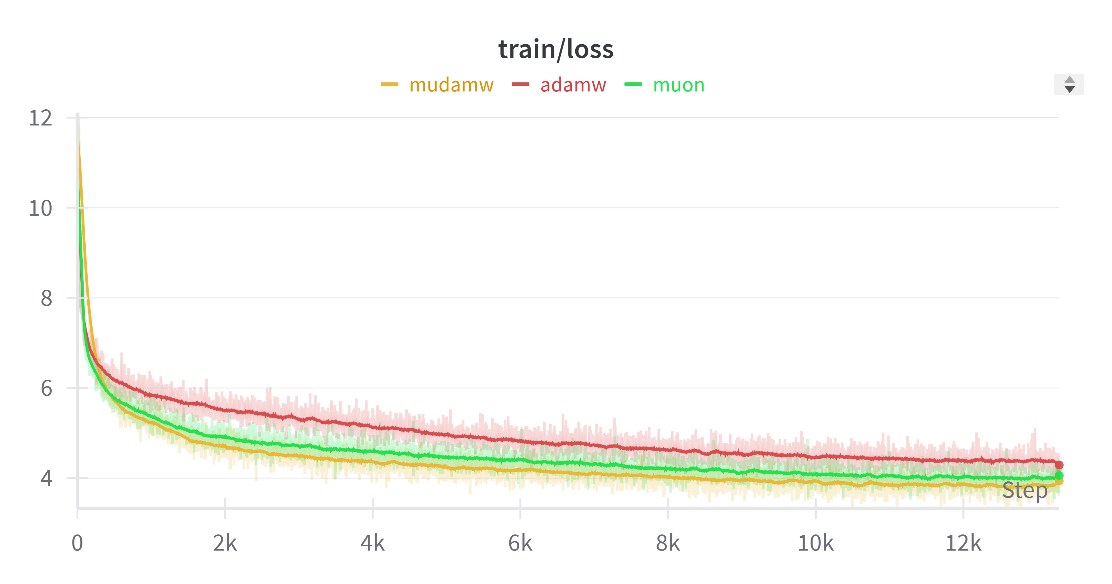 Adam+msgin appears to outperform Muon (from Twitter @KyleLiang5)
After seeing this, we also tried it on a small model, and it turned out we could reproduce a similar conclusion! So it seems that applying $\mathop{\text{msign}}$ to existing optimizers may often produce better results. This kind of manipulation is hard to explain within the original Muon framework, but here, once we understand it as (the limiting version of) singular value clipping applied to the update, this result follows naturally.
Approximate Estimation
It's generally believed that operations related to SVD (Singular Value Decomposition), such as spectral normalization, singular value clipping, or $\mathop{\text{msign}}$, are relatively expensive, so it's still worth looking for simpler forms. Since our goal is only to find the scaling law across model scales, further simplification is indeed possible.
(Note: In fact, our Moonlight work shows that with a good implementation, even applying $\mathop{\text{msign}}$ at every single update step incurs a very limited extra cost. So the content of this section is, at this point, more about exploring an explicit scaling law than about saving computation.)
Let's start again with initialization. Initialization is a one-off computation, so it's not really a problem even if it's somewhat costly — hence the earlier approach of randomly initializing and then applying spectral normalization/singular value clipping/$\mathop{\text{msign}}$ can still be kept as is. But if we want to be extra precise, we can make use of a statistical result: for an $d_{k-1}\times d_k$ matrix independently sampled i.i.d. from a standard normal distribution, its largest singular value is approximately $\sqrt{d_{k-1}} + \sqrt{d_k}$. This is equivalent to saying that as long as we change the sampling standard deviation to
\begin{equation}\sigma_k = \Theta\left(\sqrt{\frac{d_k}{d_{k-1}}}(\sqrt{d_{k-1}} + \sqrt{d_k})^{-1}\right) = \Theta\left(\sqrt{\frac{1}{d_{k-1}}\min\left(1, \frac{d_k}{d_{k-1}}\right)}\right) \label{eq:spec-std}\end{equation}
we can satisfy the requirement $\Vert\boldsymbol{W}_k\Vert_2=\Theta\left(\sqrt{\frac{d_k}{d_{k-1}}}\right)$ at initialization. For a proof of this statistical result, see references such as High-Dimensional Probability and the Marchenko-Pastur law; we won't go into it further here.
Next let's examine the update quantity, which is a bit trickier, since the spectral norm of an arbitrary update $\boldsymbol{\Phi}_k$ isn't so easy to estimate. Here we need to make use of an empirical observation: parameter gradient matrices are typically low-rank. "Low-rank" here doesn't necessarily mean mathematically strict low rank, but rather that a handful of the largest singular values (a number independent of model scale) are noticeably larger than the rest, making low-rank approximation viable. This is also the theoretical basis behind various LoRA-style optimizations.
A direct consequence of this empirical assumption is that the spectral norm and the nuclear norm become approximately comparable: the spectral norm is the largest singular value, while the nuclear norm is the sum of all singular values; and under the assumption above, the nuclear norm is approximately equal to the sum of just the top few singular values, so the two are at least of the same order, i.e., $\Theta(\Vert\nabla_{\boldsymbol{W}_k}\mathcal{L}\Vert_2)=\Theta(\Vert\nabla_{\boldsymbol{W}_k}\mathcal{L}\Vert_*)$. Next we make use of the relationship between $\Delta\mathcal{L}$ and $\Delta\boldsymbol{W}_k$:
\begin{equation}\Delta\mathcal{L} \approx \sum_k \langle \Delta\boldsymbol{W}_k, \nabla_{\boldsymbol{W}_k}\mathcal{L}\rangle_F \leq \sum_k \Vert\Delta\boldsymbol{W}_k\Vert_2\, \Vert\nabla_{\boldsymbol{W}_k}\mathcal{L}\Vert_*\end{equation}
Here $\langle\cdot,\cdot\rangle_F$ denotes the $F$ inner product, i.e., treating the flattened matrix as a vector and taking its inner product. The inequality follows from a classical matrix norm inequality $\langle\boldsymbol{A},\boldsymbol{B}\rangle_F \leq \Vert\boldsymbol{A}\Vert_2\, \Vert\boldsymbol{B}\Vert_*$, similar in spirit to the Hölder inequality — in fact, this is precisely what we proved when deriving Muon in Appreciating the Muon Optimizer: The Essential Leap from Vectors to Matrices. Based on the above and combined with the low-rank assumption on the gradient, we have
\begin{equation}\Delta\mathcal{L} \sim \sum_k \Theta(\Vert\Delta\boldsymbol{W}_k\Vert_2\, \Vert\nabla_{\boldsymbol{W}_k}\mathcal{L}\Vert_*) \sim \sum_k \Theta(\Vert\Delta\boldsymbol{W}_k\Vert_2\, \Vert\nabla_{\boldsymbol{W}_k}\mathcal{L}\Vert_2)\end{equation}
Recall that we already proved earlier that under the two spectral conditions we necessarily have $\Delta\mathcal{L}=\Theta(1)$. Combining this with the above, we obtain, when $\Vert\Delta\boldsymbol{W}_k\Vert_2=\Theta\left(\sqrt{\frac{d_k}{d_{k-1}}}\right)$,
\begin{equation}\Vert\nabla_{\boldsymbol{W}_k}\mathcal{L}\Vert_2 = \Theta\left(\sqrt{\frac{d_{k-1}}{d_k}}\right)\label{eq:grad-norm}\end{equation}
This is an important estimate for the order of magnitude of the gradient, derived directly from the two spectral conditions — avoiding any explicit gradient computation. This is the third delightful aspect of the spectral condition: it lets us obtain this kind of estimate without going through the chain rule to compute an explicit gradient expression.
Learning Rate Strategy
Applying the estimate $\eqref{eq:grad-norm}$ to SGD, i.e., $\Delta \boldsymbol{W}_k = -\eta_k \nabla_{\boldsymbol{W}_k}\mathcal{L}$, and using $\eqref{eq:grad-norm}$ we get $\Vert\nabla_{\boldsymbol{W}_k}\mathcal{L}\Vert_2=\Theta\left(\sqrt{\frac{d_{k-1}}{d_k}}\right)$. To achieve the goal $\Vert\Delta\boldsymbol{W}_k\Vert_2=\Theta\left(\sqrt{\frac{d_k}{d_{k-1}}}\right)$, we need
\begin{equation}\eta_k = \Theta\left(\frac{d_k}{d_{k-1}}\right)\label{eq:sgd-eta}\end{equation}
As for Adam, we still approximate it with SignSGD, $\newcommand{sign}{\mathop{\text{sign}}}\Delta \boldsymbol{W}_k = -\eta_k \sign(\nabla_{\boldsymbol{W}_k}\mathcal{L})$. Since $\sign$ is generally $\pm 1$, we have $\Vert\sign(\nabla_{\boldsymbol{W}_k}\mathcal{L})\Vert_F = \Theta(\sqrt{d_{k-1} d_k})$, and since $\sign$ is an element-wise operation, it generally doesn't do anything special to raise the rank, so we consider $\sign(\nabla_{\boldsymbol{W}_k}\mathcal{L})$ to be low-rank just like $\nabla_{\boldsymbol{W}_k}\mathcal{L}$. Hence, analogous to the nuclear-norm case, the $F$ norm and the spectral norm will be of the same order, i.e., $\Vert\sign(\nabla_{\boldsymbol{W}_k}\mathcal{L})\Vert_2 = \Theta(\sqrt{d_{k-1} d_k})$
So to achieve the goal $\Vert\Delta\boldsymbol{W}_k\Vert_2=\Theta\left(\sqrt{\frac{d_k}{d_{k-1}}}\right)$, we need
\begin{equation}\eta_k = \Theta\left(\frac{1}{d_{k-1}}\right)\label{eq:adam-eta}\end{equation}
We can now compare the results of the spectral condition with MuP. MuP assumes we want to build a $\mathbb{R}^{d_{in}}\mapsto\mathbb{R}^{d_{out}}$ model, dividing it into three parts: first, a $d_{in}\times d$ matrix projects the input to $d$ dimensions; then, modeling proceeds in the $d$-dimensional space, where the parameters are all $d\times d$ square matrices; and finally a $d\times d_{out}$ matrix produces a $d_{out}$-dimensional output. Correspondingly, MuP's conclusions are also divided into three parts: input, intermediate, and output.
For initialization, MuP gives the input variance as $1/d_{in}$, the output variance as $1/d^2$, and the variance of the remaining parameters as $1/d$, whereas the spectral condition's result is just the single expression $\eqref{eq:spec-std}$. But if we look closely, we'll see that $\eqref{eq:spec-std}$ already covers all three of MuP's cases: letting the input, intermediate, and output matrix sizes be $d_{in}\times d,d\times d,d\times d_{out}$, and substituting into $\eqref{eq:spec-std}$, we get
\begin{equation}\begin{aligned} \sigma_{in}^2 =&\, \Theta\left(\frac{1}{d_{in}}\min\left(1, \frac{d}{d_{in}}\right)\right) = \Theta\left(\frac{1}{d_{in}}\right) \\ \sigma_k^2 =&\, \Theta\left(\frac{1}{d}\min\left(1, \frac{d}{d}\right)\right) = \Theta\left(\frac{1}{d}\right) \\ \sigma_{out}^2 =&\, \Theta\left(\frac{1}{d}\min\left(1, \frac{d_{out}}{d}\right)\right) = \Theta\left(\frac{1}{d^2}\right) \end{aligned} \qquad(d\to\infty) \end{equation}
Readers might wonder why we're only considering $d\to\infty$. That's because $d_{in},d_{out}$ are all task-dependent numbers, essentially constants, and the only variable model scale is $d$ — since MuP studies the asymptotic behavior of hyperparameters as model scale grows, its conclusions are all understood as the simplified regime where $d$ is sufficiently large.
For learning rate, in the case of SGD, MuP's input learning rate is $d$, output learning rate is $1/d$, and the learning rate for the remaining parameters is $1$ — note that these are all proportional relationships rather than equalities — and the spectral condition's result $\eqref{eq:sgd-eta}$ likewise covers all three of these cases. Similarly, for Adam, MuP's input learning rate is $1$, output learning rate is $1/d$, and the learning rate for the remaining parameters is $1/d$; the spectral condition again describes all three cases with the single expression $\eqref{eq:adam-eta}$.
So the spectral condition, in a way that (to my mind) is simpler, produces a more concise result — and the actual content of this more concise result is richer than MuP's, because it doesn't rely on any strong assumptions about model architecture or parameter shapes. This is why I call the spectral condition a higher-order version of MuP.
Summary
This article introduced an upgraded version of MuP — the spectral condition — which analyzes the conditions for stable model training starting from inequalities related to the spectral norm, arriving at results richer than MuP's in a more convenient way.
$$\left\{\begin{aligned} &\,\text{expected property:}\left\{\begin{aligned} &\,\Vert\boldsymbol{x}_k\Vert_{RMS}=\Theta(1) \\[5pt] &\,\Vert\Delta\boldsymbol{x}_k\Vert_{RMS}=\Theta(1) \end{aligned}\right. \\[10pt] &\,\text{spectral condition:}\left\{\begin{aligned} &\,\Vert\boldsymbol{W}_k\Vert_2 = \Theta\left(\sqrt{\frac{d_k}{d_{k-1}}}\right) \\[5pt] &\,\Vert\Delta\boldsymbol{W}_k\Vert_2 = \Theta\left(\sqrt{\frac{d_k}{d_{k-1}}}\right) \end{aligned}\right. \\[10pt] &\,\text{implementation:}\left\{\begin{aligned} &\,\text{spectral norm:}\left\{\begin{aligned} &\,\boldsymbol{W}_k = \sigma\sqrt{\frac{d_k}{d_{k-1}}}\frac{\boldsymbol{W}_k'}{\Vert\boldsymbol{W}_k'\Vert_2} \\[5pt] &\,\Delta \boldsymbol{W}_k = \eta\sqrt{\frac{d_k}{d_{k-1}}}\frac{\boldsymbol{\Phi}_k}{\Vert\boldsymbol{\Phi}_k\Vert_2} \end{aligned}\right. \\[10pt] &\,\text{singular value clipping:}\left\{\begin{aligned} &\,\boldsymbol{W}_k = \sigma\sqrt{\frac{d_k}{d_{k-1}}}\mathop{\text{SVC}}(\boldsymbol{W}_k')\xrightarrow{\text{limit}} \sigma\sqrt{\frac{d_k}{d_{k-1}}}\mathop{\text{msign}}(\boldsymbol{W}_k')\\[5pt] &\,\Delta \boldsymbol{W}_k = \eta\sqrt{\frac{d_k}{d_{k-1}}}\mathop{\text{SVC}}(\boldsymbol{\Phi}_k)\xrightarrow{\text{limit}} \eta\sqrt{\frac{d_k}{d_{k-1}}}\mathop{\text{msign}}(\boldsymbol{\Phi}_k) \end{aligned}\right. \\[10pt] &\,\text{approx estimate:}\left\{\begin{aligned} &\,\sigma_k = \Theta\left(\sqrt{\frac{1}{d_{k-1}}\min\left(1, \frac{d_k}{d_{k-1}}\right)}\right) \\[5pt] &\,\eta_k = \left\{\begin{aligned} &\,\text{SGD: }\Theta\left(\frac{d_k}{d_{k-1}}\right) \\[5pt] &\,\text{Adam: }\Theta\left(\frac{1}{d_{k-1}}\right) \end{aligned}\right. \end{aligned}\right. \\[10pt] \end{aligned}\right. \end{aligned}\right.$$
Translated automatically with claude-sonnet-5; all equations are reproduced verbatim from the source. Copyright remains with the original author.