Muon Optimizer Appreciation: The Essential Leap from Vectors to Matrices
With the arrival of the LLM era, academic enthusiasm for optimizer research seems to have cooled somewhat. This is mainly because the current mainstream AdamW already satisfies most needs, while "major surgery" on optimizers requires enormous validation costs. Consequently, most current changes to optimizers are just small patches that industry applies to AdamW based on their own training experience.
However, an optimizer called "Muon" has recently been generating quite a buzz on Twitter. It claims to be more efficient than AdamW, and it's not just a "minor tweak" on top of Adam, but embodies some thought-provoking principles about the difference between vectors and matrices. Let's take a look together in this post.
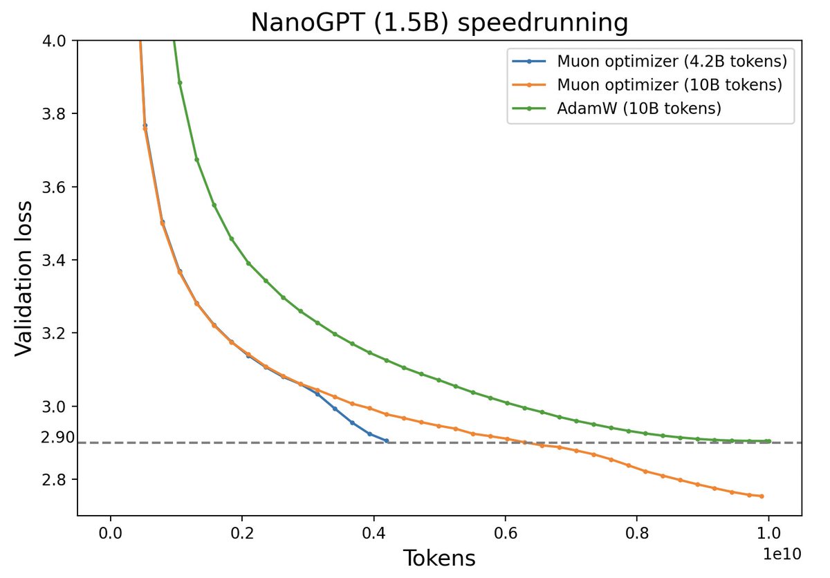 Muon vs AdamW performance comparison (source: Twitter @Yuchenj_UW)more
First look at the algorithm
Muon stands for "MomentUm Orthogonalized by Newton-schulz." It applies to matrix parameters $\boldsymbol{W}\in\mathbb{R}^{n\times m}$, and its update rule is
\begin{equation}\begin{aligned} \boldsymbol{M}_t =&\, \beta\boldsymbol{M}_{t-1} + \boldsymbol{G}_t \\[5pt] \boldsymbol{W}_t =&\, \boldsymbol{W}_{t-1} - \eta_t [\text{msign}(\boldsymbol{M}_t) + \lambda \boldsymbol{W}_{t-1}] \\ \end{aligned}\end{equation}
Here $\text{msign}$ is the matrix sign function. It is not simply applying the $\text{sign}$ operation elementwise to the matrix, but rather the matrix generalization of the $\text{sign}$ function. Its relationship to SVD is:
\begin{equation}\boldsymbol{U},\boldsymbol{\Sigma},\boldsymbol{V}^{\top} = \text{SVD}(\boldsymbol{M}) \quad\Rightarrow\quad \text{msign}(\boldsymbol{M}) = \boldsymbol{U}_{[:,:r]}\boldsymbol{V}_{[:,:r]}^{\top}\end{equation}
where $\boldsymbol{U}\in\mathbb{R}^{n\times n},\boldsymbol{\Sigma}\in\mathbb{R}^{n\times m},\boldsymbol{V}\in\mathbb{R}^{m\times m}$, and $r$ is the rank of $\boldsymbol{M}$. We'll expand on more theoretical details later; for now let's try to build an intuitive sense of the following fact:
Muon is an adaptive-learning-rate optimizer similar to Adam.
The distinguishing feature of adaptive-learning-rate optimizers such as Adagrad, RMSprop, and Adam is that they adjust the update magnitude for each parameter by dividing by the square root of a moving average of squared gradients. This achieves two effects: 1) scaling the loss function by a constant does not affect the optimization trajectory; 2) the update magnitude across parameter components is made as consistent as possible. Muon exhibits exactly these two properties:
1. If the loss function is multiplied by $\lambda$, then $\boldsymbol{M}$ is also multiplied by $\lambda$, and as a result $\boldsymbol{\Sigma}$ gets multiplied by $\lambda$; but Muon's final update turns $\boldsymbol{\Sigma}$ into the identity matrix, so this has no effect on the optimization outcome.
2. When $\boldsymbol{M}$ is decomposed via SVD as $\boldsymbol{U}\boldsymbol{\Sigma}\boldsymbol{V}^{\top}$, the different singular values of $\boldsymbol{\Sigma}$ reflect the "anisotropy" of $\boldsymbol{M}$, and setting them all to one makes it more isotropic, which also serves to synchronize update magnitudes.
By the way, regarding point 2, does this remind any reader of BERT-whitening? It should also be noted that Muon has a Nesterov variant, which simply replaces $\text{msign}(\boldsymbol{M}_t)$ in the update rule with $\text{msign}(\beta\boldsymbol{M}_t + \boldsymbol{G}_t)$, with everything else identical; for simplicity we won't go into detail here.
(Archaeology note: it turns out that the 2015 paper Stochastic Spectral Descent for Restricted Boltzmann Machines had already proposed an optimization algorithm essentially identical to Muon, calling it "Stochastic Spectral Descent" at the time.)
The sign function
Using SVD, we can also prove the identity
\begin{equation}\text{msign}(\boldsymbol{M}) = (\boldsymbol{M}\boldsymbol{M}^{\top})^{-1/2}\boldsymbol{M}= \boldsymbol{M}(\boldsymbol{M}^{\top}\boldsymbol{M})^{-1/2}\label{eq:msign-id}\end{equation}
where ${}^{-1/2}$ is the inverse of the matrix's $1/2$-th power, or the pseudo-inverse if it is not invertible. This identity helps us better understand why $\text{msign}$ is a matrix generalization of $\text{sign}$: for a scalar $x$ we have $\text{sign}(x)=x(x^2)^{-1/2}$, which is exactly a special case of the above formula (when $\boldsymbol{M}$ is a $1\times 1$ matrix). This special case can also be extended to diagonal matrices $\boldsymbol{M}=\text{diag}(\boldsymbol{m})$:
\begin{equation}\text{msign}(\boldsymbol{M}) = \text{diag}(\boldsymbol{m})[\text{diag}(\boldsymbol{m})^2]^{-1/2} = \text{diag}(\text{sign}(\boldsymbol{m}))=\text{sign}(\boldsymbol{M})\end{equation}
where $\text{sign}(\boldsymbol{m})$ and $\text{sign}(\boldsymbol{M})$ denote taking $\text{sign}$ elementwise on the vector/matrix. The above formula means that when $\boldsymbol{M}$ is diagonal, Muon degenerates into momentum-based SignSGD (Signum) or the Tiger optimizer I proposed earlier, both of which are classic approximations of Adam. Conversely, the difference between Muon and Signum/Tiger is that the elementwise $\text{sign}(\boldsymbol{M})$ is replaced by its matrix version $\text{msign}(\boldsymbol{M})$.
For an $n$-dimensional vector, we can also view it as an $n\times 1$ matrix, in which case $\text{msign}(\boldsymbol{m}) = \boldsymbol{m}/\Vert\boldsymbol{m}\Vert_2$ is exactly $l_2$-normalization. So, within the Muon framework, we have two viewpoints for vectors: one treats them as diagonal matrices, as with LayerNorm's gamma parameter, resulting in taking $\text{sign}$ of the momentum; the other treats them as $n\times 1$ matrices, resulting in $l_2$-normalization of the momentum. Additionally, although input and output embeddings are also matrices, they are used sparsely, so it makes more sense to treat them as multiple independent vectors rather than as a single matrix.
When $m=n=r$, $\text{msign}(\boldsymbol{M})$ also has the meaning of "optimal orthogonal approximation":
\begin{equation}\text{msign}(\boldsymbol{M}) = \mathop{\text{argmin}}_{\boldsymbol{O}^{\top}\boldsymbol{O} = \boldsymbol{I}}\Vert \boldsymbol{M} - \boldsymbol{O}\Vert_F^2 \label{eq:nearest-orth}\end{equation}
Similarly, for $\text{sign}(\boldsymbol{M})$ we can write (assuming $\boldsymbol{M}$ has no zero elements):
\begin{equation}\text{sign}(\boldsymbol{M}) = \mathop{\text{argmin}}_{\boldsymbol{O}\in\{-1,1\}^{n\times m}}\Vert \boldsymbol{M} - \boldsymbol{O}\Vert_F^2\end{equation}
Whether it's $\boldsymbol{O}^{\top}\boldsymbol{O} = \boldsymbol{I}$ or $\boldsymbol{O}\in\{-1,1\}^{n\times m}$, both can be viewed as a form of regularization constraint on the update. So Muon and Signum/Tiger can be seen as optimizers under the same underlying idea: they all take the momentum $\boldsymbol{M}$ as their starting point for constructing the update, but choose different regularization methods for it.
Proof of formula $\eqref{eq:nearest-orth}$: For an orthogonal matrix $\boldsymbol{O}$, we have
\begin{equation}\begin{aligned} > \Vert \boldsymbol{M} - \boldsymbol{O}\Vert_F^2 =&\, \Vert \boldsymbol{M}\Vert_F^2 + \Vert \boldsymbol{O}\Vert_F^2 - 2\langle\boldsymbol{M},\boldsymbol{O}\rangle_F \\[5pt] > =&\, \Vert \boldsymbol{M}\Vert_F^2 + n - 2\text{Tr}(\boldsymbol{M}\boldsymbol{O}^{\top})\\[5pt] > =&\, \Vert \boldsymbol{M}\Vert_F^2 + n - 2\text{Tr}(\boldsymbol{U}\boldsymbol{\Sigma}\boldsymbol{V}^{\top}\boldsymbol{O}^{\top})\\[5pt] > =&\, \Vert \boldsymbol{M}\Vert_F^2 + n - 2\text{Tr}(\boldsymbol{\Sigma}\boldsymbol{V}^{\top}\boldsymbol{O}^{\top}\boldsymbol{U})\\ > =&\, \Vert \boldsymbol{M}\Vert_F^2 + n - 2\sum_{i=1}^n \boldsymbol{\Sigma}_{i,i}(\boldsymbol{V}^{\top}\boldsymbol{O}^{\top}\boldsymbol{U})_{i,i} > \end{aligned}\end{equation}
where the operation rules involved have already been introduced in pseudo-inverse. Since $\boldsymbol{U},\boldsymbol{V},\boldsymbol{O}$ are both orthogonal matrices, $\boldsymbol{V}^{\top}\boldsymbol{O}^{\top}\boldsymbol{U}$ is also orthogonal; every entry of an orthogonal matrix is necessarily bounded by 1 in absolute value, and since $\boldsymbol{\Sigma}_{i,i} > 0$, the above expression attains its minimum when each $(\boldsymbol{V}^{\top}\boldsymbol{O}^{\top}\boldsymbol{U})_{i,i}$ attains its maximum, i.e., $(\boldsymbol{V}^{\top}\boldsymbol{O}^{\top}\boldsymbol{U})_{i,i}=1$, which implies $\boldsymbol{V}^{\top}\boldsymbol{O}^{\top}\boldsymbol{U}=\boldsymbol{I}$, i.e., $\boldsymbol{O}=\boldsymbol{U}\boldsymbol{V}^{\top}$.
This conclusion can also be carefully extended to the case where the $m,n,r$'s are not all equal, but we won't go further into that here.
Iterative solution
In practice, computing $\text{msign}(\boldsymbol{M})$ by performing SVD on $\boldsymbol{M}$ at every step would be quite expensive, so the author proposes using Newton–Schulz iteration to approximate $\text{msign}(\boldsymbol{M})$.
The starting point for the iteration is the identity $\eqref{eq:msign-id}$. Without loss of generality, assume $n\geq m$, and then consider a Taylor expansion of $(\boldsymbol{M}^{\top}\boldsymbol{M})^{-1/2}$ around $\boldsymbol{M}^{\top}\boldsymbol{M}=\boldsymbol{I}$, expanding by directly applying the result of the scalar function $t^{-1/2}$ to matrices:
\begin{equation}t^{-1/2} = 1 - \frac{1}{2}(t-1) + \frac{3}{8}(t-1)^2 - \frac{5}{16}(t-1)^3 + \cdots\end{equation}
Keeping terms up to second order gives $(15 - 10t + 3t^2)/8$, so we have
\begin{equation}\text{msign}(\boldsymbol{M}) = \boldsymbol{M}(\boldsymbol{M}^{\top}\boldsymbol{M})^{-1/2}\approx \frac{15}{8}\boldsymbol{M} - \frac{5}{4}\boldsymbol{M}(\boldsymbol{M}^{\top}\boldsymbol{M}) + \frac{3}{8}\boldsymbol{M}(\boldsymbol{M}^{\top}\boldsymbol{M})^2\end{equation}
If $\boldsymbol{X}_t$ is some approximation of $\text{msign}(\boldsymbol{M})$, we believe that substituting it into the above expression yields a better approximation of $\text{msign}(\boldsymbol{M})$, giving us a usable iteration scheme:
\begin{equation}\boldsymbol{X}_{t+1} = \frac{15}{8}\boldsymbol{X}_t - \frac{5}{4}\boldsymbol{X}_t(\boldsymbol{X}_t^{\top}\boldsymbol{X}_t) + \frac{3}{8}\boldsymbol{X}_t(\boldsymbol{X}_t^{\top}\boldsymbol{X}_t)^2\end{equation}
However, if we look at Muon's official code, we find that the Newton–Schulz iteration inside indeed has this form, but the three coefficients are $(3.4445, -4.7750, 2.0315)$, and the author gives no mathematical derivation—only a rather cryptic comment:
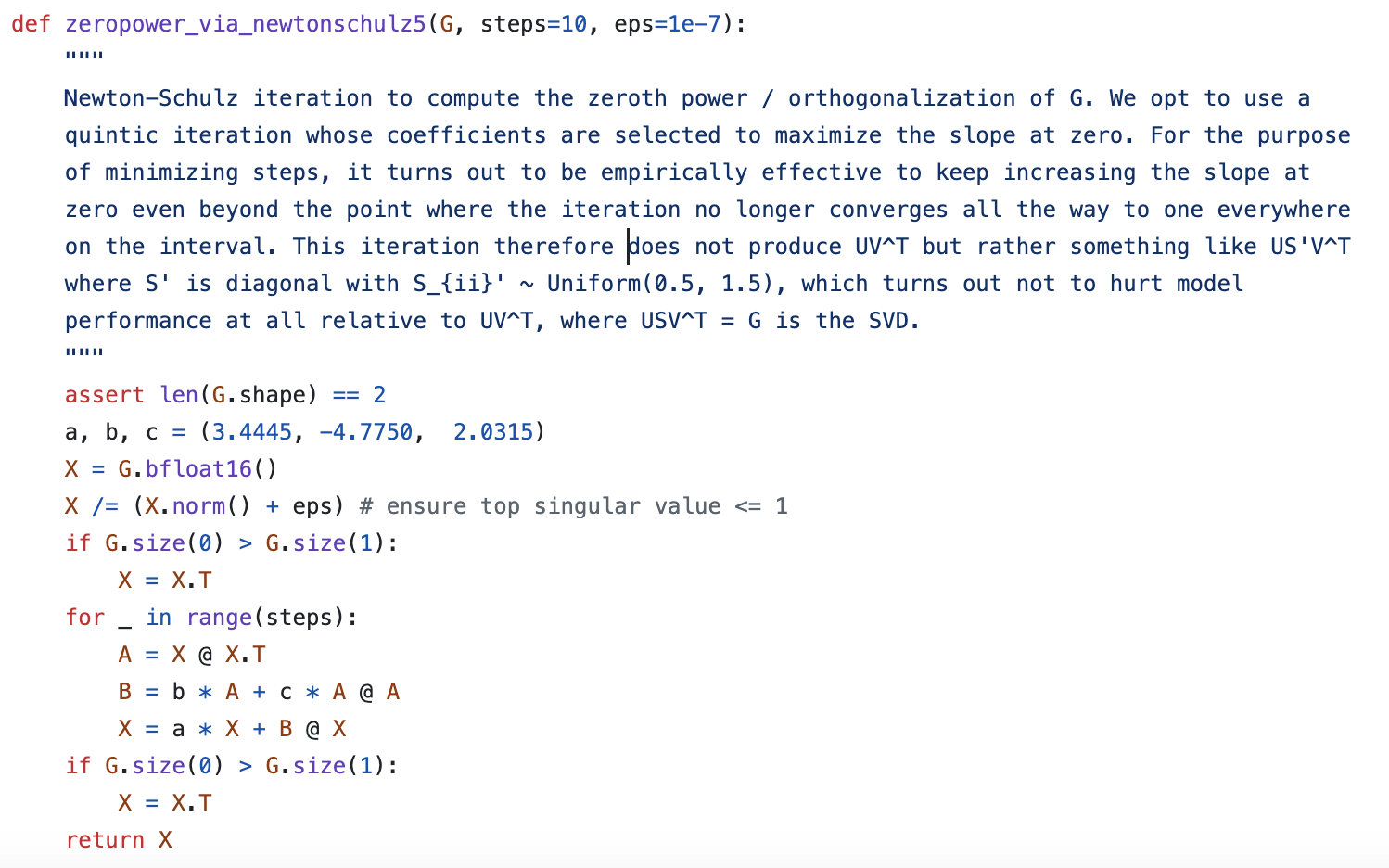 Newton-Schulz iteration in the Muon optimizer
Accelerating convergence
To guess where the official iteration algorithm came from, let's consider the general iteration process
\begin{equation}\boldsymbol{X}_{t+1} = a\boldsymbol{X}_t + b\boldsymbol{X}_t(\boldsymbol{X}_t^{\top}\boldsymbol{X}_t) + c\boldsymbol{X}_t(\boldsymbol{X}_t^{\top}\boldsymbol{X}_t)^2\label{eq:iteration}\end{equation}
where $a,b,c$ are three coefficients to be solved for. If we want a higher-order iterative algorithm, we can also add terms like $\boldsymbol{X}_t(\boldsymbol{X}_t^{\top}\boldsymbol{X}_t)^3$, $\boldsymbol{X}_t(\boldsymbol{X}_t^{\top}\boldsymbol{X}_t)^4$, etc. one by one—the analysis that follows applies generally.
We choose the initial value $\boldsymbol{X}_0=\boldsymbol{M}/\Vert\boldsymbol{M}\Vert_F$, where $\Vert\cdot\Vert_F$ is the matrix's $F$-norm; the reasoning is that dividing by $\Vert\boldsymbol{M}\Vert_F$ doesn't change the SVD's $\boldsymbol{U},\boldsymbol{V}$, but ensures that all singular values of $\boldsymbol{X}_0$ lie within $[0,1]$, giving the iteration a more standardized starting point. Now suppose $\boldsymbol{X}_t$ can be decomposed via SVD as $\boldsymbol{U}\boldsymbol{\Sigma}_t\boldsymbol{V}^{\top}$; substituting into the above formula we get
\begin{equation}\boldsymbol{X}_{t+1} = \boldsymbol{U}_{[:,:r]}(a \boldsymbol{\Sigma}_{t,[:r,:r]} + b \boldsymbol{\Sigma}_{t,[:r,:r]}^3 + c \boldsymbol{\Sigma}_{t,[:r,:r]}^5)\boldsymbol{V}_{[:,:r]}^{\top}\end{equation}
Thus, formula $\eqref{eq:iteration}$ effectively iterates the diagonal matrix $\boldsymbol{\Sigma}_{[:r,:r]}$ formed from the singular values. If we write $\boldsymbol{X}_t=\boldsymbol{U}_{[:,:r]}\boldsymbol{\Sigma}_{t,[:r,:r]}\boldsymbol{V}_{[:,:r]}^{\top}$, then we have $\boldsymbol{\Sigma}_{t+1,[:r,:r]} = g(\boldsymbol{\Sigma}_{t,[:r,:r]})$, where $g(x) = ax + bx^3 + cx^5$. And since the power of a diagonal matrix is just taking the power of each diagonal element separately, the problem reduces to iterating a single singular value $\sigma$. Our goal is to compute $\boldsymbol{U}_{[:,:r]}\boldsymbol{V}_{[:,:r]}^{\top}$, in other words, we want the iteration to turn $\boldsymbol{\Sigma}_{[:r,:r]}$ into the identity matrix, which can be further reduced to iterating $\sigma_{t+1} = g(\sigma_t)$ so as to turn a single singular value into 1.
Inspired by @leloykun, we treat the choice of $a,b,c$ as an optimization problem, with the goal of making the iteration converge as fast as possible for any initial singular value. First, we reparametrize $g(x)$ as
\begin{equation}g(x) = x + \kappa x(x^2 - x_1^2)(x^2 - x_2^2)\end{equation}
where $x_1 \leq x_2$. The benefit of this parametrization is that it directly exposes the 5 fixed points of the iteration $0,\pm x_1,\pm x_2$. Since our goal is convergence to 1, we choose the initialization $x_1 < 1,x_2 > 1$, with the idea that regardless of whether the iteration moves toward $x_1$ or toward $x_2$, the result ends up near 1.
Next, we fix the number of iteration steps $T$, turning the iteration process into a deterministic function; then, having fixed the shape of the matrix (i.e., $n,m$), we can sample a batch of matrices and compute their singular values via SVD. Finally, taking these singular values as inputs with a target output of 1 and a squared-error loss function, the whole model becomes fully differentiable and can be optimized with gradient descent (@leloykun instead assumed $x_1 + x_2 = 2$ and used grid search to solve it).
Some computed results:
$$\begin{array}{ccc|ccc|ccc|c|c} \hline n & m & T & \kappa & x_1 & x_2 & a & b & c & \text{mse} & \text{mse}_{\text{o}}\\ \hline 1024 & 1024 & 3 & 7.020 & 0.830 & 0.830 & 4.328 & -9.666 & 7.020 & 0.10257 & 0.18278 \\ 1024 & 1024 & 5 & 1.724 & 0.935 & 1.235 & 3.297 & -4.136 & 1.724 & 0.02733 & 0.04431 \\ 2048 & 1024 & 3 & 7.028 & 0.815 & 0.815 & 4.095 & -9.327 & 7.028 & 0.01628 & 0.06171 \\ 2048 & 1024 & 5 & 1.476 & 0.983 & 1.074 & 2.644 & -3.128 & 1.476 & 0.00038 & 0.02954 \\ 4096 & 1024 & 3 & 6.948 & 0.802 & 0.804 & 3.886 & -8.956 & 6.948 & 0.00371 & 0.02574 \\ 4096 & 1024 & 5 & 1.214 & 1.047 & 1.048 & 2.461 & -2.663 & 1.214 & 0.00008 & 0.02563 \\ \hline 2048 & 2048 & 3 & 11.130 & 0.767 & 0.767 & 4.857 & -13.103 & 11.130 & 0.10739 & 0.24410 \\ 2048 & 2048 & 5 & 1.779 & 0.921 & 1.243 & 3.333 & -4.259 & 1.779 & 0.03516 & 0.04991 \\ 4096 & 4096 & 3 & 18.017 & 0.705 & 0.705 & 5.460 & -17.929 & 18.017 & 0.11303 & 0.33404 \\ 4096 & 4096 & 5 & 2.057 & 0.894 & 1.201 & 3.373 & -4.613 & 2.057 & 0.04700 & 0.06372 \\ 8192 & 8192 & 3 & 30.147 & 0.643 & 0.643 & 6.139 & -24.893 & 30.147 & 0.11944 & 0.44843 \\ 8192 & 8192 & 5 & 2.310 & 0.871 & 1.168 & 3.389 & -4.902 & 2.310 & 0.05869 & 0.07606 \\ \hline \end{array}$$
Here $\text{mse}_{\text{o}}$ is the result computed by Muon's author's $a,b,c$. The table shows a clear dependence on both matrix size and number of iteration steps; in terms of the loss function, non-square matrices converge more easily than square ones; the $a,b,c$ given by Muon's author is roughly the optimal solution for square matrices at 5 iteration steps. When the number of iteration steps is fixed, the result depends on the matrix size, which fundamentally reflects the distribution of singular values—a noteworthy fact about this distribution is that when $n,m\to\infty$, it follows the Marchenko–Pastur distribution.
Reference code:
import jax
import jax.numpy as jnp
from tqdm import tqdm

n, m, T = 1024, 1024, 5
key, data = jax.random.key(42), jnp.array([])
for _ in tqdm(range(1000), ncols=0, desc='SVD'):
    key, subkey = jax.random.split(key)
    M = jax.random.normal(subkey, shape=(n, m))
    S = jnp.linalg.svd(M, full_matrices=False)[1]
    data = jnp.concatenate([data, S / (S**2).sum()**0.5])

@jax.jit
def f(w, x):
    k, x1, x2 = w
    for _ in range(T):
        x = x + k * x * (x**2 - x1**2) * (x**2 - x2**2)
    return ((x - 1)**2).mean()

f_grad = jax.grad(f)
w, u = jnp.array([1, 0.9, 1.1]), jnp.zeros(3)
for _ in tqdm(range(100000), ncols=0, desc='SGD'):
    u = 0.9 * u + f_grad(w, data)  # 动量加速
    w = w - 0.01 * u

k, x1, x2 = w
a, b, c = 1 + k * x1**2 * x2**2, -k * (x1**2 + x2**2), k
print(f'{n} & {m} & {T} & {k:.3f} & {x1:.3f} & {x2:.3f} & {a:.3f} & {b:.3f} & {c:.3f} & {f(w, data):.5f}')
Some reflections
With the default choice of $T=5$, for a matrix parameter of size $n\times n$, each Muon update step requires at least 15 matrix multiplications between $n\times n$ and $n\times n$-sized matrices—undoubtedly a heavier computational load than Adam. This might make some readers worry whether Muon is practical in real settings.
In fact, such worries are unwarranted. Although Muon's computation is more complex than Adam's, the added time per step is small—my own conclusion is under 5%, and Muon's author claims to achieve as little as 2%. This is because Muon's matrix multiplications happen after the current gradient is computed but before the next gradient computation, during which almost all compute is otherwise idle; moreover, these matrix multiplications are of static size and can be parallelized, so they don't meaningfully increase the time cost. On the contrary, Muon requires one fewer set of cached variables than Adam, so its memory cost is actually lower.
What's most thought-provoking about Muon is really the intrinsic distinction between vectors and matrices, and its impact on optimization. Common optimizers like SGD, Adam, and Tiger have elementwise update rules—that is, regardless of whether the parameter is a vector or a matrix, it's effectively treated as one large vector, and each component is updated independently according to the same rule. Optimizers with this property tend to be theoretically simpler to analyze, and are also convenient for tensor parallelism, since splitting a large matrix into two independent smaller matrices doesn't change the optimization trajectory.
But Muon is different: it treats the matrix as the fundamental unit and takes into account some of the matrix's unique properties. Some readers might find this puzzling: aren't matrices and vectors both just arrangements of numbers—what difference could there be? Here's an example: for matrices we have the notion of "trace," the sum of the diagonal elements. This concept isn't arbitrary—it has the important property of being invariant under similarity transformations, and it also equals the sum of all the matrix's eigenvalues. This example already shows that the diagonal elements of a matrix are not, in fact, on entirely equal footing with the off-diagonal elements. It is precisely by accounting for this asymmetry that Muon achieves better performance.
Of course, this also brings some downsides. If a matrix is split across different devices, then with Muon we need to aggregate the gradients before computing the update, rather than updating each device's shard independently—this increases communication cost. Even setting parallelism aside, this issue exists elsewhere too: for instance, multi-head attention typically projects to $Q$ (and similarly for $K,V$) via a single large matrix, then obtains multiple heads via reshaping. This means the model parameters contain only a single matrix, but it is essentially several small matrices in disguise, so strictly speaking we ought to split the large matrix into independent smaller matrices for updating.
In short, Muon's non-elementwise update rule, while capturing the essential difference between vectors and matrices, also introduces some minor complications—which may not sit well with every reader's aesthetic sensibilities.
(Addendum: almost simultaneously with this blog post's publication, Muon's author Keller Jordan also published his own post, Muon: An optimizer for hidden layers in neural networks.)
A norm-based perspective
Theoretically speaking, what key property of matrices does Muon actually capture? Perhaps the norm-based perspective that follows can answer this question.
This section's discussion draws mainly on the papers Stochastic Spectral Descent for Discrete Graphical Models and Old Optimizer, New Norm: An Anthology, especially the latter. That said, the starting point isn't new—we already touched on it briefly in Gradient Flow: Exploring the Path to the Minimum: for a vector parameter $\boldsymbol{w}\in\mathbb{R}^n$, we define the next update rule as
\begin{equation}\boldsymbol{w}_{t+1} = \mathop{\text{argmin}}_{\boldsymbol{w}} \frac{\Vert\boldsymbol{w} - \boldsymbol{w}_t\Vert^2}{2\eta_t} + \mathcal{L}(\boldsymbol{w})\end{equation}
where $\Vert\Vert$ is some vector norm—this is called "steepest gradient descent" under a given norm constraint. Next, assuming $\eta_t$ is sufficiently small, the first term dominates, meaning $\boldsymbol{w}_{t+1}$ and $\boldsymbol{w}_t$ will be close, so we assume a first-order approximation of $\mathcal{L}(\boldsymbol{w})$ suffices, and the problem reduces to
\begin{equation}\boldsymbol{w}_{t+1} = \mathop{\text{argmin}}_{\boldsymbol{w}} \frac{\Vert\boldsymbol{w} - \boldsymbol{w}_t\Vert^2}{2\eta_t} + \mathcal{L}(\boldsymbol{w}_t) + \nabla_{\boldsymbol{w}_t}\mathcal{L}(\boldsymbol{w}_t)^{\top}(\boldsymbol{w}-\boldsymbol{w}_t)\end{equation}
Writing $\Delta\boldsymbol{w}_{t+1} = \boldsymbol{w}_{t+1}-\boldsymbol{w}_t, \boldsymbol{g}_t = \nabla_{\boldsymbol{w}_t}\mathcal{L}(\boldsymbol{w}_t)$, this can be abbreviated as
\begin{equation}\Delta\boldsymbol{w}_{t+1} = \mathop{\text{argmin}}_{\Delta\boldsymbol{w}} \frac{\Vert\Delta\boldsymbol{w}\Vert^2}{2\eta_t} + \boldsymbol{g}_t^{\top}\Delta\boldsymbol{w}\end{equation}
The usual approach to computing $\Delta\boldsymbol{w}_{t+1}$ is via differentiation, but Old Optimizer, New Norm: An Anthology offers a unified scheme that avoids taking derivatives: decompose $\Delta\boldsymbol{w}$ into its norm $\gamma = \Vert\Delta\boldsymbol{w}\Vert$ and direction vector $\boldsymbol{\varphi} = -\Delta\boldsymbol{w}/\Vert\Delta\boldsymbol{w}\Vert$, giving
\begin{equation}\min_{\Delta\boldsymbol{w}} \frac{\Vert\Delta\boldsymbol{w}\Vert^2}{2\eta_t} + \boldsymbol{g}_t^{\top}\Delta\boldsymbol{w} = \min_{\gamma\geq 0, \Vert\boldsymbol{\varphi}\Vert=1} \frac{\gamma^2}{2\eta_t} - \gamma\boldsymbol{g}_t^{\top}\boldsymbol{\varphi} = \min_{\gamma\geq 0} \frac{\gamma^2}{2\eta_t} - \gamma\bigg(\underbrace{\max_{\Vert\boldsymbol{\varphi}\Vert=1}\boldsymbol{g}_t^{\top}\boldsymbol{\varphi}}_{\text{denote}\Vert \boldsymbol{g}_t\Vert^{\dagger}}\bigg)\end{equation}
$\gamma$ is just a scalar, similar to a learning rate, and it's easy to find its optimal value $\eta_t\Vert \boldsymbol{g}_t\Vert^{\dagger}$; the update direction is the $\boldsymbol{\varphi}^*$ that maximizes $\boldsymbol{g}_t^{\top}\boldsymbol{\varphi}$ ($\Vert\boldsymbol{\varphi}\Vert=1$). Substituting the Euclidean norm, i.e. $\Vert\boldsymbol{\varphi}\Vert_2 = \sqrt{\boldsymbol{\varphi}^{\top}\boldsymbol{\varphi}}$, gives us $\Vert \boldsymbol{g}_t\Vert^{\dagger}=\Vert \boldsymbol{g}_t\Vert_2$ and $\boldsymbol{\varphi}^* = \boldsymbol{g}_t/\Vert\boldsymbol{g}_t\Vert_2$, so $\Delta\boldsymbol{w}_{t+1}=-\eta_t \boldsymbol{g}_t$—i.e., gradient descent (SGD). More generally, for the $p$-norm
\begin{equation}\Vert\boldsymbol{\varphi}\Vert_p = \sqrt[\uproot{10}p]{\sum_{i=1}^n |\varphi_i|^p}\end{equation}Hölder's inequality gives $\boldsymbol{g}^{\top}\boldsymbol{\varphi} \leq \Vert \boldsymbol{g}\Vert_q \Vert \boldsymbol{\varphi}\Vert_p$, where $1/p + 1/q = 1$, and using it we get
\begin{equation}\max_{\Vert\boldsymbol{\varphi}\Vert_p=1}\boldsymbol{g}^{\top}\boldsymbol{\varphi} = \Vert \boldsymbol{g}\Vert_q\end{equation}
with equality holding under the condition
\begin{equation}\boldsymbol{\varphi}^* = \frac{1}{\Vert\boldsymbol{g}\Vert_q^{q/p}}\Big[\text{sign}(g_1) |g_1|^{q/p},\text{sign}(g_2) |g_2|^{q/p},\cdots,\text{sign}(g_n) |g_n|^{q/p}\Big]\end{equation}
The optimizer using this as its direction vector is called pbSGD; see pbSGD: Powered Stochastic Gradient Descent Methods for Accelerated Non-Convex Optimization. In particular, when $p\to\infty$, we have $q\to 1$ and $|g_i|^{q/p}\to 1$, which degenerates to SignSGD—meaning SignSGD is in fact the steepest gradient descent under the $\Vert\Vert_{\infty}$-norm.
Matrix norms
Now let's turn to matrix parameters $\boldsymbol{W}\in\mathbb{R}^{n\times m}$. Similarly, we define its update rule as
\begin{equation}\boldsymbol{W}_{t+1} = \mathop{\text{argmin}}_{\boldsymbol{W}} \frac{\Vert\boldsymbol{W} - \boldsymbol{W}_t\Vert^2}{2\eta_t} + \mathcal{L}(\boldsymbol{W})\end{equation}
where $\Vert\Vert$ is some matrix norm. Using the same first-order approximation, we obtain
\begin{equation}\Delta\boldsymbol{W}_{t+1} = \mathop{\text{argmin}}_{\Delta\boldsymbol{W}} \frac{\Vert\Delta\boldsymbol{W}\Vert^2}{2\eta_t} + \text{Tr}(\boldsymbol{G}_t^{\top}\Delta\boldsymbol{W})\end{equation}
where $\Delta\boldsymbol{W}_{t+1} = \boldsymbol{W}_{t+1}-\boldsymbol{W}_t, \boldsymbol{G}_t = \nabla_{\boldsymbol{W}_t}\mathcal{L}(\boldsymbol{W}_t)$. Again using the "norm-direction" decoupling, i.e. setting $\gamma = \Vert\Delta\boldsymbol{w}\Vert$ and $\boldsymbol{\Phi} = -\Delta\boldsymbol{W}/\Vert\Delta\boldsymbol{W}\Vert$, we get
\begin{equation}\min_{\Delta\boldsymbol{W}} \frac{\Vert\Delta\boldsymbol{W}\Vert^2}{2\eta_t} + \text{Tr}(\boldsymbol{G}_t^{\top}\Delta\boldsymbol{W}) = \min_{\gamma\geq 0} \frac{\gamma^2}{2\eta_t} - \gamma\bigg(\underbrace{\max_{\Vert\boldsymbol{\Phi}\Vert=1}\text{Tr}(\boldsymbol{G}_t^{\top}\boldsymbol{\Phi})}_{\text{denote}\Vert \boldsymbol{G}_t\Vert^{\dagger}}\bigg)\end{equation}
From here, the analysis depends on the specific norm. There are two commonly used matrix norms: one is the Frobenius norm, which is essentially the Euclidean norm computed after flattening the matrix into a vector—in this case the conclusion is the same as for vectors, giving SGD as the answer, so we won't dwell on it further. The other is the $2$-norm (also called the spectral norm) induced by a vector norm:
\begin{equation}\Vert \boldsymbol{\Phi}\Vert_2 = \max_{\Vert \boldsymbol{x}\Vert_2 = 1} \Vert \boldsymbol{\Phi}\boldsymbol{x}\Vert_2\end{equation}
Note that the $\Vert\Vert_2$ operations on the right-hand side act on vectors, so this is well-defined. For more discussion of the $2$-norm, see Lipschitz Constraints in Deep Learning: Generalization and Generative Models and The Road to Low-Rank Approximation (II): SVD. Since the $2$-norm is induced by "matrix-vector" multiplication, it fits matrix multiplication more naturally, and it always satisfies $\Vert\boldsymbol{\Phi}\Vert_2\leq \Vert\boldsymbol{\Phi}\Vert_F$—meaning the $2$-norm is tighter than the $F$-norm.
So, let's proceed with the computation for the $2$-norm. Let the SVD of $\boldsymbol{G}$ be $\boldsymbol{U}\boldsymbol{\Sigma}\boldsymbol{V}^{\top} = \sum\limits_{i=1}^r \sigma_i \boldsymbol{u}_i \boldsymbol{v}_i^{\top}$; we then have
\begin{equation}\text{Tr}(\boldsymbol{G}^{\top}\boldsymbol{\Phi})=\text{Tr}\Big(\sum_{i=1}^r \sigma_i \boldsymbol{v}_i \boldsymbol{u}_i^{\top}\boldsymbol{\Phi}\Big) = \sum_{i=1}^r \sigma_i \boldsymbol{u}_i^{\top}\boldsymbol{\Phi}\boldsymbol{v}_i\end{equation}
By definition, when $\Vert\boldsymbol{\Phi}\Vert_2=1$ we have $\Vert\boldsymbol{\Phi}\boldsymbol{v}_i\Vert_2\leq \Vert\boldsymbol{v}_i\Vert_2=1$, hence $\boldsymbol{u}_i^{\top}\boldsymbol{\Phi}\boldsymbol{v}_i\leq 1$, and thus
\begin{equation}\text{Tr}(\boldsymbol{G}^{\top}\boldsymbol{\Phi})\leq \sum_{i=1}^r \sigma_i\end{equation}
Equality is attained when all the $\boldsymbol{u}_i^{\top}\boldsymbol{\Phi}\boldsymbol{v}_i$ equal 1, in which case
\begin{equation}\boldsymbol{\Phi} = \sum_{i=1}^r \boldsymbol{u}_i \boldsymbol{v}_i^{\top} = \boldsymbol{U}_{[:,:r]}\boldsymbol{V}_{[:,:r]}^{\top} = \text{msign}(\boldsymbol{G})\end{equation}
We have thus shown that gradient descent under the $2$-norm penalty is exactly the Muon optimizer when $\beta=0$! When $\beta > 0$, the moving average kicks in, and we can regard it as a more accurate estimate of the gradient, so we instead take $\text{msign}$ of the momentum. In summary, Muon is equivalent to gradient descent under the $2$-norm constraint; the $2$-norm better captures the essential differences between matrices, allowing each step to be more precise and more fundamentally grounded.
Tracing the origins
Muon has an even older related work, Shampoo: Preconditioned Stochastic Tensor Optimization, a 2018 paper proposing the Shampoo optimizer, which shares a similar spirit with Muon.
The strategy of Adam—using the average of squared gradients to adapt the learning rate—was first proposed in the Adagrad paper Adaptive Subgradient Methods for Online Learning and Stochastic Optimization, which proposed directly accumulating squared gradients, equivalent to a global equally-weighted average. Later, RMSProp and Adam adapted the design of momentum, switching to a moving average instead, which proved to work better in practice.
Moreover, what Adagrad originally proposed was actually accumulating the outer product $\boldsymbol{g}\boldsymbol{g}^{\top}$; it's just that caching the outer product is too costly in space, so in practice it's replaced with the Hadamard product $\boldsymbol{g}\odot\boldsymbol{g}$. So what's the theoretical basis for accumulating outer products? We derived this in Viewing Adaptive Learning Rate Optimizers through Hessian Approximation: the answer is that "the long-term average of gradient outer products $\mathbb{E}[\boldsymbol{g}\boldsymbol{g}^{\top}]$ approximates the square of the Hessian matrix $\sigma^2\boldsymbol{\mathcal{H}}_{\boldsymbol{\theta}^*}^2$," so this is actually approximating Newton's second-order method.
Shampoo inherits Adagrad's idea of caching outer products, but strikes a compromise given the cost issue. Like Muon, it also optimizes for matrices (and higher-order tensors); its strategy is to cache the matrix products $\boldsymbol{G}\boldsymbol{G}^{\top}$ and $\boldsymbol{G}^{\top}\boldsymbol{G}$ of the gradients, rather than the outer product itself, so the space cost becomes $\mathcal{O}(n^2 + m^2)$ instead of $\mathcal{O}(n^2 m^2)$:
\begin{equation}\begin{aligned} \boldsymbol{L}_t =&\, \beta\boldsymbol{L}_{t-1} + \boldsymbol{G}_t\boldsymbol{G}_t^{\top} \\[5pt] \boldsymbol{R}_t =&\, \beta\boldsymbol{R}_{t-1} + \boldsymbol{G}_t^{\top}\boldsymbol{G}_t \\[5pt] \boldsymbol{W}_t =&\, \boldsymbol{W}_{t-1} - \eta_t \boldsymbol{L}_t^{-1/4}\boldsymbol{G}_t\boldsymbol{R}_t^{-1/4} \\ \end{aligned}\end{equation}
Here, the $\beta$ is something I've added myself—Shampoo by default assumes $\beta=1$. ${}^{-1/4}$ is likewise a matrix power operation that can be computed via SVD. Since Shampoo doesn't propose any Newton–Schulz-style approximation and instead computes it directly via SVD, to save computational cost it doesn't recompute $\boldsymbol{L}_t^{-1/4}$ and $\boldsymbol{R}_t^{-1/4}$ at every single step, but rather updates their results only every fixed number of steps.
In particular, when $\beta=0$, Shampoo's update vector is $(\boldsymbol{G}\boldsymbol{G}^{\top})^{-1/4}\boldsymbol{G}(\boldsymbol{G}^{\top}\boldsymbol{G})^{-1/4}$, and by performing an SVD on $\boldsymbol{G}$, we can show that
\begin{equation}(\boldsymbol{G}\boldsymbol{G}^{\top})^{-1/4}\boldsymbol{G}(\boldsymbol{G}^{\top}\boldsymbol{G})^{-1/4} = (\boldsymbol{G}\boldsymbol{G}^{\top})^{-1/2}\boldsymbol{G}= \boldsymbol{G}(\boldsymbol{G}^{\top}\boldsymbol{G})^{-1/2}=\text{msign}(\boldsymbol{G})\end{equation}
This shows that when $\beta=0$, Shampoo and Muon are theoretically equivalent! Thus, Shampoo and Muon share common ground in the design of their update rules.
Summary
This post introduced the Muon optimizer, which has been generating quite a buzz on Twitter recently. Custom-designed for matrix parameters, it currently appears more efficient than AdamW, and seems to capture some essential differences between vectorization and matrixization that are well worth studying and reflecting on.
Translated automatically with claude-sonnet-5; all equations are reproduced verbatim from the source. Copyright remains with the original author.