The Road to Low-Rank Approximation (II): SVD
In the previous post we introduced the "pseudoinverse", which concerns the optimal solution of the objective $\Vert \boldsymbol{A}\boldsymbol{B} - \boldsymbol{M}\Vert_F^2$ when the matrices $\boldsymbol{M}$ and $\boldsymbol{A}$ (or $\boldsymbol{B}$) are given. In this post we turn to the case where $\boldsymbol{A},\boldsymbol{B}$ are not given at all, i.e., the optimal solution of
\begin{equation}\mathop{\text{argmin}}_{\boldsymbol{A},\boldsymbol{B}}\Vert \boldsymbol{A}\boldsymbol{B} - \boldsymbol{M}\Vert_F^2\label{eq:loss-ab}\end{equation}
where $\boldsymbol{A}\in\mathbb{R}^{n\times r}, \boldsymbol{B}\in\mathbb{R}^{r\times m}, \boldsymbol{M}\in\mathbb{R}^{n\times m},r < \min(n,m)$. Put plainly, this amounts to finding the "optimal $r$-rank approximation (the best approximation with rank not exceeding $r$)" of the matrix $\boldsymbol{M}$. To solve this problem, we need to bring in the famous "SVD (Singular Value Decomposition)". Although this series opened with the pseudoinverse, its "fame" is nowhere near that of SVD — plenty of people have heard of, and even used, SVD without ever hearing of the pseudoinverse. The author himself learned about SVD first and only later came across the pseudoinverse.
In what follows, we will introduce SVD by centering the discussion around the optimal low-rank approximation of a matrix.
A First Look at the Conclusion
For any matrix $\boldsymbol{M}\in\mathbb{R}^{n\times m}$, one can always find a decomposition of the following form, called the Singular Value Decomposition (SVD):
\begin{equation}\boldsymbol{M} = \boldsymbol{U}\boldsymbol{\Sigma} \boldsymbol{V}^{\top}\end{equation}more
where $\boldsymbol{U}\in\mathbb{R}^{n\times n},\boldsymbol{V}\in\mathbb{R}^{m\times m}$ are both orthogonal matrices, and $\boldsymbol{\Sigma}\in\mathbb{R}^{n\times m}$ is a nonnegative diagonal matrix:
\begin{equation}\boldsymbol{\Sigma}_{i,j} = \left\{\begin{aligned}&\sigma_i, &i = j \\ &0,&i \neq j\end{aligned}\right.\end{equation}
By convention the diagonal entries are sorted in decreasing order, i.e., $\sigma_1\geq \sigma_2\geq\sigma_3\geq\cdots\geq 0$; these diagonal entries are called singular values. From a numerical computation point of view, we can keep only the nonzero entries of $\boldsymbol{\Sigma}$, reducing the size of $\boldsymbol{U},\boldsymbol{\Sigma},\boldsymbol{V}$ to $n\times r, r\times r, m\times r$ (where $r$ is the rank of $\boldsymbol{M}$); keeping the full orthogonal matrices, however, is more convenient for theoretical analysis.
SVD also holds for complex matrices, but then the orthogonal matrices must be replaced by unitary matrices and the transpose by the conjugate transpose. Here, though, we mainly focus on the real-matrix case, which is more relevant to machine learning. The basic theory of SVD — existence, computation methods, and its connection to optimal low-rank approximation — is what we'll cover below, presented in the author's own way of understanding it.
In the two-dimensional plane, SVD has a very intuitive geometric meaning. A 2D orthogonal matrix is essentially a rotation (plus possibly a reflection, though we can be a bit loose about that for the sake of geometric intuition), so $\boldsymbol{M}\boldsymbol{x}=\boldsymbol{U}\boldsymbol{\Sigma} \boldsymbol{V}^{\top}\boldsymbol{x}$ means that any linear transformation applied to a (column) vector $x$ can be decomposed into three steps: rotation, stretching, and rotation again, as shown in the figure below:
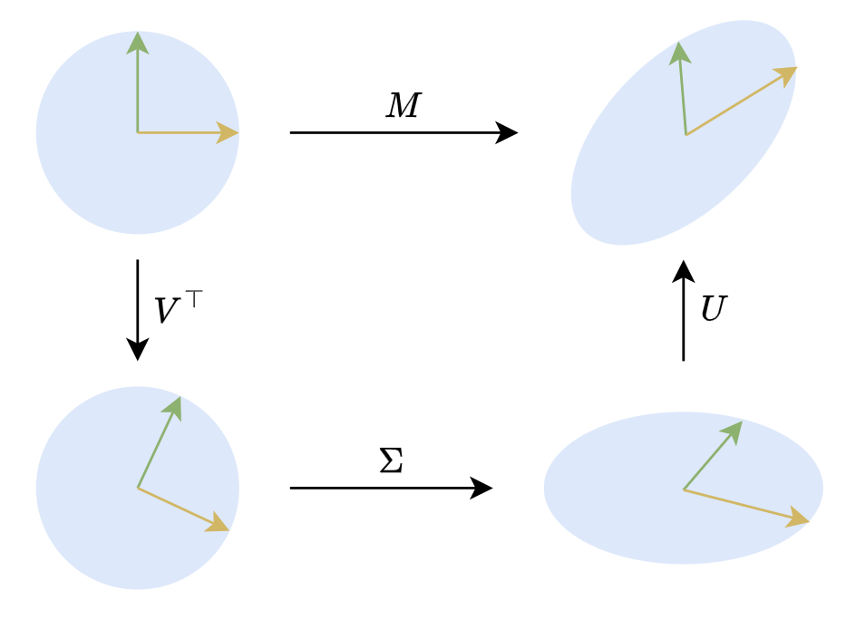 Geometric meaning of SVD
Some Applications
Whether for theoretical analysis or numerical computation, SVD has extremely broad applications. One of the underlying reasons is that the commonly used matrix/vector norms are invariant under orthogonal transformations, so the SVD structure — an orthogonal matrix on each side sandwiching a diagonal matrix in the middle — can often be used to convert many matrix-related optimization objectives into equivalent special cases involving a nonnegative diagonal matrix, thereby simplifying the problem.
General Formula for the Pseudoinverse
Take the pseudoinverse as an example. When $\boldsymbol{A}\in\mathbb{R}^{n\times r}$ has rank $r$, we have
\begin{equation}\boldsymbol{A}^{\dagger} = \mathop{\text{argmin}}_{\boldsymbol{B}\in\mathbb{R}^{r\times n}}\Vert \boldsymbol{A}\boldsymbol{B} - \boldsymbol{I}_n\Vert_F^2\end{equation}
In the previous post we derived the expression for $\boldsymbol{A}^{\dagger}$ via differentiation, and then spent some effort extending it to the case where the rank of $\boldsymbol{A}$ is less than $r$. But if we bring in SVD, the problem becomes much simpler. We can decompose $\boldsymbol{A}$ as $\boldsymbol{U}\boldsymbol{\Sigma} \boldsymbol{V}^{\top}$, and then write $\boldsymbol{B}$ as $\boldsymbol{V} \boldsymbol{Z} \boldsymbol{U}^{\top}$ — note that we haven't required $\boldsymbol{Z}$ to be diagonal, so $\boldsymbol{B}=\boldsymbol{V} \boldsymbol{Z} \boldsymbol{U}^{\top}$ can always be achieved — giving us
\begin{equation}\begin{aligned} \min_\boldsymbol{B}\Vert \boldsymbol{A}\boldsymbol{B} - \boldsymbol{I}_n\Vert_F^2 =&\, \min_\boldsymbol{Z}\Vert \boldsymbol{U}\boldsymbol{\Sigma} \boldsymbol{V}^{\top}\boldsymbol{V} \boldsymbol{Z} \boldsymbol{U}^{\top} - \boldsymbol{I}_n\Vert_F^2 \\ =&\, \min_\boldsymbol{Z}\Vert \boldsymbol{U}(\boldsymbol{\Sigma} \boldsymbol{Z} - \boldsymbol{I}_n) \boldsymbol{U}^{\top}\Vert_F^2 \\ =&\, \min_\boldsymbol{Z}\Vert \boldsymbol{\Sigma} \boldsymbol{Z} - \boldsymbol{I}_n\Vert_F^2 \end{aligned}\end{equation}
The last equality relies on the result we proved in the previous post: "orthogonal transformations do not change the $F$-norm." This reduces the problem to finding the pseudoinverse of the diagonal matrix $\boldsymbol{\Sigma}$. We can then write $\boldsymbol{\Sigma} \boldsymbol{Z} - \boldsymbol{I}_n$ in block-matrix form as
\begin{equation}\begin{aligned}\boldsymbol{\Sigma} \boldsymbol{Z} - \boldsymbol{I}_n =&\, \begin{pmatrix}\boldsymbol{\Sigma}_{[:r,:r]} \\ \boldsymbol{0}_{(n-r)\times r}\end{pmatrix} \begin{pmatrix}\boldsymbol{Z}_{[:r,:r]} & \boldsymbol{Z}_{[:r,r:]}\end{pmatrix} - \begin{pmatrix}\boldsymbol{I}_r & \boldsymbol{0}_{r\times(n-r)} \\ \boldsymbol{0}_{(n-r)\times r} & \boldsymbol{I}_{n-r}\end{pmatrix} \\ =&\, \begin{pmatrix}\boldsymbol{\Sigma}_{[:r,:r]}\boldsymbol{Z}_{[:r,:r]} - \boldsymbol{I}_r & \boldsymbol{\Sigma}_{[:r,:r]}\boldsymbol{Z}_{[:r,r:]}\\ \boldsymbol{0}_{(n-r)\times r} & -\boldsymbol{I}_{n-r}\end{pmatrix} \end{aligned}\end{equation}
Here the slicing should be understood following Python array conventions. From this final form, we can see that to minimize the $F$-norm of $\boldsymbol{\Sigma} \boldsymbol{Z} - \boldsymbol{I}_n$, the unique solution is $\boldsymbol{Z}_{[:r,:r]}=\boldsymbol{\Sigma}_{[:r,:r]}^{-1}$, $\boldsymbol{Z}_{[:r,r:]}=\boldsymbol{0}_{r\times(n-r)}$. In other words, $\boldsymbol{Z}$ is obtained by taking the reciprocal of every nonzero entry of $\boldsymbol{\Sigma}^{\top}$ and then transposing; we denote it as $\boldsymbol{\Sigma}^{\dagger}$. Thus, under SVD we have
\begin{equation}\boldsymbol{A}=\boldsymbol{U}\boldsymbol{\Sigma} \boldsymbol{V}^{\top}\quad\Rightarrow\quad \boldsymbol{A}^{\dagger} = \boldsymbol{V}\boldsymbol{\Sigma}^{\dagger}\boldsymbol{U}^{\top}\end{equation}
One can further show that this result also holds when the rank of $\boldsymbol{A}$ is less than $r$, so it is a fully general formula — indeed, some textbooks take it directly as the definition of the pseudoinverse. We can also observe that this formula does not distinguish between the left and right pseudoinverse, which tells us that the left pseudoinverse and right pseudoinverse of the same matrix coincide, so there's no need to specifically distinguish "left" from "right" when talking about the pseudoinverse.
Matrix Norms
Using the fact that orthogonal transformations preserve the $F$-norm, we can also obtain
\begin{equation}\Vert \boldsymbol{M}\Vert_F^2 = \Vert \boldsymbol{U}\boldsymbol{\Sigma} \boldsymbol{V}^{\top}\Vert_F^2 = \Vert \boldsymbol{\Sigma} \Vert_F^2 = \sum_{i=1}^{\min(n,m)}\sigma_i^2\end{equation}
That is, the sum of the squared singular values equals the square of the $F$-norm. Besides the $F$-norm, SVD can also be used to compute the "spectral norm." In the previous post we mentioned that the $F$-norm is just one kind of matrix norm; another commonly used matrix norm is the spectral norm, induced from a vector norm, defined as:
\begin{equation}\Vert \boldsymbol{M}\Vert_2 = \max_{\Vert \boldsymbol{x}\Vert = 1} \Vert \boldsymbol{M}\boldsymbol{x}\Vert\end{equation}
Note that the norms appearing on the right-hand side of the equation are vector norms (magnitudes, the $2$-norm), so the definition above is well-defined. Since it is induced by the vector $2$-norm, it is also called the $2$-norm of the matrix. Numerically, the spectral norm of a matrix equals its largest singular value, i.e., $\Vert \boldsymbol{M}\Vert_2 = \sigma_1$. To prove this, we simply take the SVD of $\boldsymbol{M}$ as $\boldsymbol{U}\boldsymbol{\Sigma} \boldsymbol{V}^{\top}$, and substitute into the definition of the spectral norm:
\begin{equation}\max_{\Vert \boldsymbol{x}\Vert = 1} \Vert \boldsymbol{M}\boldsymbol{x}\Vert = \max_{\Vert \boldsymbol{x}\Vert = 1} \Vert \boldsymbol{U}\boldsymbol{\Sigma} (\boldsymbol{V}^{\top}\boldsymbol{x})\Vert = \max_{\Vert \boldsymbol{y}\Vert = 1} \Vert \boldsymbol{\Sigma} \boldsymbol{y}\Vert\end{equation}
The second equality again uses the fact that orthogonal matrices preserve vector norms. Now the problem reduces to the spectral norm of the diagonal matrix $\boldsymbol{\Sigma}$, which is straightforward: letting $\boldsymbol{y} = (y_1,y_2,\cdots,y_m)$, we have
\begin{equation}\Vert \boldsymbol{\Sigma} \boldsymbol{y}\Vert^2 = \sum_{i=1}^m \sigma_i^2 y_i^2 \leq \sum_{i=1}^m \sigma_1^2 y_i^2 = \sigma_1^2\sum_{i=1}^m y_i^2 = \sigma_1^2\end{equation}
so $\Vert \boldsymbol{\Sigma} \boldsymbol{y}\Vert$ never exceeds $\sigma_1$, with equality achieved when $\boldsymbol{y}=(1,0,\cdots,0)$, hence $\Vert \boldsymbol{M}\Vert_2=\sigma_1$. Comparing with the result for the $F$-norm, we can also see that $\Vert \boldsymbol{M}\Vert_2\leq \Vert \boldsymbol{M}\Vert_F$ always holds.
Low-Rank Approximation
Finally, let's return to the main topic of this post — the optimal low-rank approximation, i.e., the objective $\eqref{eq:loss-ab}$. Decomposing $\boldsymbol{M}$ as $\boldsymbol{U}\boldsymbol{\Sigma} \boldsymbol{V}^{\top}$, we can write
\begin{equation}\begin{aligned} \Vert \boldsymbol{A}\boldsymbol{B} - \boldsymbol{M}\Vert_F^2 =&\, \Vert \boldsymbol{U}\boldsymbol{U}^{\top}\boldsymbol{A}\boldsymbol{B}\boldsymbol{V}\boldsymbol{V}^{\top} - \boldsymbol{U}\boldsymbol{\Sigma} \boldsymbol{V}^{\top}\Vert_F^2 \\ =&\, \Vert \boldsymbol{U}(\boldsymbol{U}^{\top}\boldsymbol{A}\boldsymbol{B}\boldsymbol{V} - \boldsymbol{\Sigma}) \boldsymbol{V}^{\top}\Vert_F^2 \\ =&\, \Vert \boldsymbol{U}^{\top}\boldsymbol{A}\boldsymbol{B}\boldsymbol{V} - \boldsymbol{\Sigma}\Vert_F^2 \end{aligned}\end{equation}
Note that $\boldsymbol{U}^{\top}\boldsymbol{A}\boldsymbol{B}\boldsymbol{V}$ can still represent any matrix of rank not exceeding $r$, so through SVD we have reduced the optimal $r$-rank approximation of the matrix $\boldsymbol{M}$ to the optimal $r$-rank approximation of the nonnegative diagonal matrix $\boldsymbol{\Sigma}$.
In "Matching Full Fine-Tuning! The Most Exciting LoRA Improvement I've Seen (Part 1)" we used the same idea to solve a similar optimization problem:
\begin{equation}\mathop{\text{argmin}}_{\boldsymbol{A},\boldsymbol{B}} \Vert \boldsymbol{A}\boldsymbol{A}^{\top}\boldsymbol{M} + \boldsymbol{M}\boldsymbol{B}^{\top}\boldsymbol{B} - \boldsymbol{M}\Vert_F^2\end{equation}
Using SVD and the fact that orthogonal transformations preserve the $F$-norm, we get
\begin{equation}\begin{aligned} &\,\Vert \boldsymbol{A}\boldsymbol{A}^{\top}\boldsymbol{M} + \boldsymbol{M}\boldsymbol{B}^{\top}\boldsymbol{B} - \boldsymbol{M}\Vert_F^2 \\ =&\, \Vert \boldsymbol{A}\boldsymbol{A}^{\top}\boldsymbol{U}\boldsymbol{\Sigma} \boldsymbol{V}^{\top} + \boldsymbol{U}\boldsymbol{\Sigma} \boldsymbol{V}^{\top}\boldsymbol{B}^{\top}\boldsymbol{B} - \boldsymbol{U}\boldsymbol{\Sigma} \boldsymbol{V}^{\top}\Vert_F^2 \\ =&\, \Vert \boldsymbol{U}\boldsymbol{U}^{\top}\boldsymbol{A}\boldsymbol{A}^{\top}\boldsymbol{U}\boldsymbol{\Sigma} \boldsymbol{V}^{\top} + \boldsymbol{U}\boldsymbol{\Sigma} \boldsymbol{V}^{\top}\boldsymbol{B}^{\top}\boldsymbol{B}\boldsymbol{V}\boldsymbol{V}^{\top} - \boldsymbol{U}\boldsymbol{\Sigma} \boldsymbol{V}^{\top}\Vert_F^2 \\ =&\, \Vert \boldsymbol{U}[(\boldsymbol{U}^{\top}\boldsymbol{A})(\boldsymbol{U}^{\top}\boldsymbol{A})^{\top}\boldsymbol{\Sigma} + \boldsymbol{\Sigma} (\boldsymbol{B}\boldsymbol{V})^{\top} (\boldsymbol{B}\boldsymbol{V}) - \boldsymbol{\Sigma}] \boldsymbol{V}^{\top}\Vert_F^2 \\ =&\, \Vert (\boldsymbol{U}^{\top}\boldsymbol{A})(\boldsymbol{U}^{\top}\boldsymbol{A})^{\top}\boldsymbol{\Sigma} + \boldsymbol{\Sigma} (\boldsymbol{B}\boldsymbol{V})^{\top} (\boldsymbol{B}\boldsymbol{V}) - \boldsymbol{\Sigma}\Vert_F^2 \\ \end{aligned}\end{equation}
This turns the optimization problem for a general matrix $\boldsymbol{M}$ into the special case where $\boldsymbol{M}$ is a nonnegative diagonal matrix, reducing the difficulty of the analysis. Note that if the rank of $\boldsymbol{A},\boldsymbol{B}$ does not exceed $r$, then the rank of $\boldsymbol{A}\boldsymbol{A}^{\top}\boldsymbol{M} + \boldsymbol{M}\boldsymbol{B}^{\top}\boldsymbol{B}$ is at most $2r$ (assuming $2r < \min(n,m)$), so the original problem is also asking for the optimal $2r$-rank approximation of $\boldsymbol{M}$; once converted to a nonnegative diagonal matrix, it becomes finding the optimal $2r$-rank approximation of a nonnegative diagonal matrix, which is essentially the same problem as before.
Theoretical Foundations
Having established the usefulness of SVD, we now need to fill in some theoretical proofs. First we need to guarantee the existence of SVD, and second we need to identify at least one method of computing it, so that all the applications of SVD are actually feasible. We will next resolve both issues together, using the same line of reasoning.
The Spectral Theorem
Before doing so, we need to introduce the "spectral theorem," which can be seen either as a special case of SVD or as its foundation:
Spectral Theorem For any real symmetric matrix $\boldsymbol{M}\in\mathbb{R}^{n\times n}$, there exists a spectral decomposition (also called eigenvalue decomposition)
\begin{equation}\boldsymbol{M} = \boldsymbol{U}\boldsymbol{\Lambda} \boldsymbol{U}^{\top}\end{equation}
where $\boldsymbol{U},\boldsymbol{\Lambda}\in\mathbb{R}^{n\times n}$, $\boldsymbol{U}$ is an orthogonal matrix, and $\boldsymbol{\Lambda}=\text{diag}(\lambda_1,\cdots,\lambda_n)$ is a diagonal matrix.
Put plainly, the spectral theorem asserts that any real symmetric matrix can be diagonalized by an orthogonal matrix, and this rests on two properties:
1. The eigenvalues and eigenvectors of a real symmetric matrix are all real;
2. Eigenvectors of a real symmetric matrix corresponding to different eigenvalues are orthogonal.
The proofs of these two properties are actually quite simple, so we won't go into them here. Based on these two facts we can immediately conclude that if the real symmetric matrix $\boldsymbol{M}$ has $n$ distinct eigenvalues, then the spectral theorem holds:
\begin{equation}\begin{aligned} \boldsymbol{M}\boldsymbol{u}_1 = \lambda_1 \boldsymbol{u}_1 \\ \boldsymbol{M}\boldsymbol{u}_2 = \lambda_2 \boldsymbol{u}_2\\ \vdots \\ \boldsymbol{M}\boldsymbol{u}_n = \lambda_n \boldsymbol{u}_n\end{aligned} \quad\Rightarrow\quad \boldsymbol{M}\underbrace{(\boldsymbol{u}_1, \boldsymbol{u}_2, \cdots, \boldsymbol{u}_n)}_\boldsymbol{U} = \underbrace{(\boldsymbol{u}_1, \boldsymbol{u}_2, \cdots, \boldsymbol{u}_n)}_\boldsymbol{U}\underbrace{\begin{pmatrix}\lambda_1 & 0 & \cdots & 0 \\ 0 & \lambda_2 & \cdots & 0 \\ \vdots & \vdots & \ddots & \vdots \\ 0 & 0 & \cdots & \lambda_n \\ \end{pmatrix}}_{\boldsymbol{\Lambda}}\end{equation}
where $\lambda_1,\lambda_2,\cdots,\lambda_n$ are the eigenvalues and $\boldsymbol{u}_1,\boldsymbol{u}_2,\cdots,\boldsymbol{u}_n$ the corresponding unit eigenvectors (as column vectors); written in matrix form this is $\boldsymbol{M}\boldsymbol{U}=\boldsymbol{U}\boldsymbol{\Lambda}$, so $\boldsymbol{M} = \boldsymbol{U}\boldsymbol{\Lambda} \boldsymbol{U}^{\top}$. The difficulty in the proof lies in extending this to the case of repeated eigenvalues, but before working through the full proof, let's get a feel — in a not-quite-rigorous way — for why the result for distinct eigenvalues must extend to the general case.
Why can we say this? From a numerical perspective, the probability of two real numbers being exactly equal is essentially zero, so there's practically no need to worry about the case of equal eigenvalues; put more mathematically, real matrices with distinct eigenvalues are dense within the set of all real matrices, so we can always find a family of matrices $\boldsymbol{M}_{\epsilon}$ such that when $\epsilon > 0$ its eigenvalues are pairwise distinct, and when $\epsilon \to 0$ it equals $\boldsymbol{M}$. This way, every $\boldsymbol{M}_{\epsilon}$ can be decomposed as $\boldsymbol{U}_{\epsilon}\boldsymbol{\Lambda} _{\epsilon}\boldsymbol{U}_{\epsilon}^{\top}$, and taking $\epsilon\to 0$ gives us the spectral decomposition of $\boldsymbol{M}$.
Mathematical Induction
Unfortunately, the argument above can only serve as an intuitive but non-rigorous way of understanding things, since turning it into a rigorous proof is actually quite hard. In fact, the simplest way to rigorously prove the spectral theorem is probably mathematical induction: assuming the spectral theorem holds for any real symmetric matrix of order $n-1$, we prove that it also holds for order $\boldsymbol{M}$.
The key idea of the proof is to split $\boldsymbol{M}$ into one eigenvector direction and its $n-1$-dimensional orthogonal complement, so that the induction hypothesis can be applied. Specifically, let $\lambda_1$ be a nonzero eigenvalue of $\boldsymbol{M}$, and $\boldsymbol{u}_1$ the corresponding unit eigenvector, so that $\boldsymbol{M}\boldsymbol{u}_1 = \lambda_1 \boldsymbol{u}_1$. We can supplement this with $n-1$ unit vectors orthogonal to $\boldsymbol{u}_1$, denoted $\boldsymbol{Q}=(\boldsymbol{q}_2,\cdots,\boldsymbol{q}_n)$, such that $(\boldsymbol{u}_1,\boldsymbol{q}_2,\cdots,\boldsymbol{q}_n)=(\boldsymbol{u}_1,\boldsymbol{Q})$ forms an orthogonal matrix. Now consider
\begin{equation}(\boldsymbol{u}_1,\boldsymbol{Q})^{\top} \boldsymbol{M} (\boldsymbol{u}_1, \boldsymbol{Q}) = \begin{pmatrix}\boldsymbol{u}_1^{\top} \boldsymbol{M} \boldsymbol{u}_1 & \boldsymbol{u}_1^{\top} \boldsymbol{M} \boldsymbol{Q} \\ \boldsymbol{Q}^{\top} \boldsymbol{M} \boldsymbol{u}_1 & \boldsymbol{Q}^{\top} \boldsymbol{M} \boldsymbol{Q}\end{pmatrix} = \begin{pmatrix}\lambda_1 & \boldsymbol{0}_{1\times (n-1)} \\ \boldsymbol{0}_{(n-1)\times 1} & \boldsymbol{Q}^{\top} \boldsymbol{M} \boldsymbol{Q}\end{pmatrix}\end{equation}
Note that $\boldsymbol{Q}^{\top} \boldsymbol{M} \boldsymbol{Q}$ is a square matrix of order $n-1$, and clearly a real symmetric matrix, so by the induction hypothesis it admits a spectral decomposition $\boldsymbol{V} \boldsymbol{\Lambda}_2 \boldsymbol{V}^{\top}$, where $\boldsymbol{V}$ is an orthogonal matrix of order $n-1$ and $\boldsymbol{\Lambda}_2$ is a diagonal matrix of order $n-1$; from this we get $(\boldsymbol{Q}\boldsymbol{V})^{\top} \boldsymbol{M} \boldsymbol{Q}\boldsymbol{V}= \boldsymbol{\Lambda}_2$. Based on this result, consider $\boldsymbol{U} = (\boldsymbol{u}_1, \boldsymbol{Q}\boldsymbol{V})$, which can be verified to also be an orthogonal matrix, and moreover
\begin{equation}\boldsymbol{U}^{\top}\boldsymbol{M} \boldsymbol{U} = (\boldsymbol{u}_1,\boldsymbol{Q}\boldsymbol{V})^{\top} \boldsymbol{M} (\boldsymbol{u}_1, \boldsymbol{Q}\boldsymbol{V}) = \begin{pmatrix}\lambda_1 & \boldsymbol{0}_{1\times (n-1)} \\ \boldsymbol{0}_{(n-1)\times 1} & \boldsymbol{\Lambda}_2\end{pmatrix}\end{equation}
That is, $\boldsymbol{U}$ is precisely the orthogonal matrix that diagonalizes $\boldsymbol{M}$, so $\boldsymbol{M}$ admits a spectral decomposition. This completes the crucial step of the induction.
Singular Decomposition
At this point, all the preparations are in place, and we can formally prove the existence of SVD, giving a practical method of computing it along the way.
In the previous section we introduced the spectral decomposition; it's not hard to notice its resemblance to SVD, but there are also two obvious differences: 1) the spectral decomposition applies only to real symmetric matrices, while SVD applies to any real matrix; 2) the diagonal matrix $\boldsymbol{\Sigma}$ in SVD is nonnegative, whereas the $\boldsymbol{\Lambda}$ in a spectral decomposition need not be. So what exactly is the relationship between them? It's easy to check that if the SVD of $\boldsymbol{M}$ is $\boldsymbol{U}\boldsymbol{\Sigma} \boldsymbol{V}^{\top}$, then
\begin{equation}\begin{aligned} \boldsymbol{M}\boldsymbol{M}^{\top} = \boldsymbol{U}\boldsymbol{\Sigma} \boldsymbol{V}^{\top}\boldsymbol{V}\boldsymbol{\Sigma}^{\top} \boldsymbol{U}^{\top} = \boldsymbol{U}\boldsymbol{\Sigma}\boldsymbol{\Sigma}^{\top} \boldsymbol{U}^{\top}\\ \boldsymbol{M}^{\top}\boldsymbol{M} = \boldsymbol{V}\boldsymbol{\Sigma}^{\top} \boldsymbol{U}^{\top}\boldsymbol{U}\boldsymbol{\Sigma} \boldsymbol{V}^{\top} = \boldsymbol{V}\boldsymbol{\Sigma}^{\top}\boldsymbol{\Sigma} \boldsymbol{V}^{\top}\\ \end{aligned}\end{equation}
Notice that both $\boldsymbol{\Sigma}\boldsymbol{\Sigma}^{\top}$ and $\boldsymbol{\Sigma}^{\top}\boldsymbol{\Sigma}$ are diagonal matrices, which means the spectral decompositions of $\boldsymbol{M}\boldsymbol{M}^{\top}$ and $\boldsymbol{M}^{\top}\boldsymbol{M}$ are $\boldsymbol{U}\boldsymbol{\Sigma}^2 \boldsymbol{U}^{\top}$ and $\boldsymbol{V}\boldsymbol{\Sigma}^2 \boldsymbol{V}^{\top}$ respectively. It seems, then, that computing the spectral decompositions of $\boldsymbol{M}\boldsymbol{M}^{\top}$ and $\boldsymbol{M}^{\top}\boldsymbol{M}$ separately would give us the SVD of $\boldsymbol{M}$? That's indeed correct, and it can serve as one way to compute the SVD — but we cannot directly use it to prove that the resulting $\boldsymbol{U},\boldsymbol{\Sigma},\boldsymbol{V}$ satisfies $\boldsymbol{M}=\boldsymbol{U}\boldsymbol{\Sigma} \boldsymbol{V}^{\top}$.
The key to resolving this is to take the spectral decomposition of only one of $\boldsymbol{M}\boldsymbol{M}^{\top}$ or $\boldsymbol{M}^{\top}\boldsymbol{M}$, and construct the orthogonal matrix on the other side through a different method. Without loss of generality, suppose $\boldsymbol{M}$ has rank $r \leq m$, and consider taking the spectral decomposition of $\boldsymbol{M}^{\top}\boldsymbol{M}$ as $\boldsymbol{V}\boldsymbol{\Lambda} \boldsymbol{V}^{\top}$. Note that $\boldsymbol{M}^{\top}\boldsymbol{M}$ is positive semi-definite, so $\boldsymbol{\Lambda}$ is nonnegative; assuming the diagonal entries are already sorted in decreasing order, rank $r$ means only the first $r$ entries of $\lambda_i$ are greater than zero. We define
\begin{equation}\boldsymbol{\Sigma}_{[:r,:r]} = (\boldsymbol{\Lambda}_{[:r,:r]})^{1/2},\quad \boldsymbol{U}_{[:n,:r]} = \boldsymbol{M}\boldsymbol{V}_{[:m,:r]}\boldsymbol{\Sigma}_{[:r,:r]}^{-1}\end{equation}
We can verify that
\begin{equation}\begin{aligned} \boldsymbol{U}_{[:n,:r]}^{\top}\boldsymbol{U}_{[:n,:r]} =&\, \boldsymbol{\Sigma}_{[:r,:r]}^{-1}\boldsymbol{V}_{[:m,:r]}^{\top} \boldsymbol{M}^{\top}\boldsymbol{M}\boldsymbol{V}_{[:m,:r]}\boldsymbol{\Sigma}_{[:r,:r]}^{-1} \\ =&\, \boldsymbol{\Sigma}_{[:r,:r]}^{-1}\boldsymbol{V}_{[:m,:r]}^{\top} \boldsymbol{V}\boldsymbol{\Lambda} \boldsymbol{V}^{\top}\boldsymbol{V}_{[:m,:r]}\boldsymbol{\Sigma}_{[:r,:r]}^{-1} \\ =&\, \boldsymbol{\Sigma}_{[:r,:r]}^{-1}\boldsymbol{I}_{[:r,:m]}\boldsymbol{\Lambda} \boldsymbol{I}_{[:m,:r]}\boldsymbol{\Sigma}_{[:r,:r]}^{-1} \\ =&\, \boldsymbol{\Sigma}_{[:r,:r]}^{-1}\boldsymbol{\Lambda}_{[:r,:r]}\boldsymbol{\Sigma}_{[:r,:r]}^{-1} \\ =&\, \boldsymbol{I}_r \\ \end{aligned}\end{equation}
Here we adopt the convention that slicing takes priority over transpose, inverse, and other matrix operations, i.e., $\boldsymbol{U}_{[:n,:r]}^{\top}=(\boldsymbol{U}_{[:n,:r]})^{\top}$, $\boldsymbol{\Sigma}_{[:r,:r]}^{-1}=(\boldsymbol{\Sigma}_{[:r,:r]})^{-1}$, etc. This result shows that $\boldsymbol{U}_{[:n,:r]}$ forms part of an orthogonal matrix. Next, we have
\begin{equation}\boldsymbol{U}_{[:n,:r]}\boldsymbol{\Sigma}_{[:r,:r]}\boldsymbol{V}_{[:m,:r]}^{\top} = \boldsymbol{M}\boldsymbol{V}_{[:m,:r]}\boldsymbol{\Sigma}_{[:r,:r]}^{-1}\boldsymbol{\Sigma}_{[:r,:r]}\boldsymbol{V}_{[:m,:r]}^{\top} = \boldsymbol{M}\boldsymbol{V}_{[:m,:r]}\boldsymbol{V}_{[:m,:r]}^{\top}\end{equation}
Note that $\boldsymbol{M}\boldsymbol{V}\boldsymbol{V}^{\top} = \boldsymbol{M}$ always holds, and $\boldsymbol{V}_{[:m,:r]}$ consists of the first $r$ columns of $\boldsymbol{V}$; from $\boldsymbol{M}^{\top}\boldsymbol{M}=\boldsymbol{V}\boldsymbol{\Lambda} \boldsymbol{V}^{\top}$ we can write $(\boldsymbol{M}\boldsymbol{V})^{\top}\boldsymbol{M}\boldsymbol{V} = \boldsymbol{\Lambda}$. Denoting $\boldsymbol{V}=(\boldsymbol{v}_1,\boldsymbol{v}_2,\cdots,\boldsymbol{v}_m)$, we then have $\Vert \boldsymbol{M}\boldsymbol{v}_i\Vert^2=\lambda_i$. Because of the rank condition $r$, when $i > r$ we have $\lambda_i=0$, which means that in this case $\boldsymbol{M}\boldsymbol{v}_i$ is actually the zero vector, so
\begin{equation}\begin{aligned}\boldsymbol{M} = \boldsymbol{M}\boldsymbol{V}\boldsymbol{V}^{\top} =&\, (\boldsymbol{M}\boldsymbol{V}_{[:m,:r]}, \boldsymbol{M}\boldsymbol{V}_{[:m,r:]})\begin{pmatrix}\boldsymbol{V}_{[:m,:r]}^{\top} \\ \boldsymbol{V}_{[:m,r:]}^{\top}\end{pmatrix} \\[8pt] =&\, (\boldsymbol{M}\boldsymbol{V}_{[:m,:r]}, \boldsymbol{0}_{m\times(m-r)} )\begin{pmatrix}\boldsymbol{V}_{[:m,:r]}^{\top} \\ \boldsymbol{V}_{[:m,r:]}^{\top}\end{pmatrix}\\[8pt] =&\, \boldsymbol{M}\boldsymbol{V}_{[:m,:r]}\boldsymbol{V}_{[:m,:r]}^{\top} \end{aligned}\end{equation}
This shows that $\boldsymbol{U}_{[:n,:r]}\boldsymbol{\Sigma}_{[:r,:r]}\boldsymbol{V}_{[:m,:r]}^{\top}=\boldsymbol{M}$; combined with the fact that $\boldsymbol{U}_{[:n,:r]}$ is part of an orthogonal matrix, we've already obtained the key part of the SVD of $\boldsymbol{M}$. We only need to pad $\boldsymbol{\Sigma}_{[:r,:r]}$ with zeros to size $n\times m$, giving $\boldsymbol{\Sigma}$, and extend $\boldsymbol{U}_{[:n,:r]}$ to a full $n\times n$ orthogonal matrix $\boldsymbol{U}$, and we obtain the complete SVD form $\boldsymbol{M}=\boldsymbol{U}\boldsymbol{\Sigma} \boldsymbol{V}^{\top}$.
The Approximation Theorem
Finally, let's not forget that our ultimate goal is the optimization problem $\eqref{eq:loss-ab}$ posed at the start. Now that we have SVD, we can give the answer:
If the SVD of $\boldsymbol{M}\in\mathbb{R}^{n\times m}$ is $\boldsymbol{U}\boldsymbol{\Sigma} \boldsymbol{V}^{\top}$, then the optimal $r$-rank approximation of $\boldsymbol{M}$ is $\boldsymbol{U}_{[:n,:r]}\boldsymbol{\Sigma}_{[:r,:r]} \boldsymbol{V}_{[:m,:r]}^{\top}$.
This is known as the Eckart-Young-Mirsky theorem. In the section on applications of SVD, "Low-Rank Approximation", we showed that SVD lets us reduce the optimal $r$-rank approximation problem of a general matrix to the $r$-rank approximation of a nonnegative diagonal matrix. So the Eckart-Young-Mirsky theorem amounts to saying that the optimal $r$-rank approximation of a nonnegative diagonal matrix is simply the matrix obtained by keeping only its $r$ largest diagonal entries.
Some readers might think, "Isn't this obviously true?" But the truth is that, while the conclusion is very intuitive, it is indeed not obviously true. Let's now focus on solving:
\begin{equation}\min_{\boldsymbol{A},\boldsymbol{B}}\Vert \boldsymbol{A}\boldsymbol{B} - \boldsymbol{\Sigma}\Vert_F^2\end{equation}
where $\boldsymbol{A}\in\mathbb{R}^{n\times r}, \boldsymbol{B}\in\mathbb{R}^{r\times m}, \boldsymbol{\Sigma}\in\mathbb{R}^{n\times m},r < \min(n,m)$. If we're given $\boldsymbol{A}$, the optimal solution for $\boldsymbol{B}$ has already been derived in the previous post, and it is $\boldsymbol{A}^{\dagger} \boldsymbol{\Sigma}$, so we have
\begin{equation}\min_{\boldsymbol{A},\boldsymbol{B}}\Vert \boldsymbol{A}\boldsymbol{B} - \boldsymbol{\Sigma}\Vert_F^2 = \min_\boldsymbol{A}\Vert (\boldsymbol{A}\boldsymbol{A}^{\dagger} - \boldsymbol{I}_n)\boldsymbol{\Sigma}\Vert_F^2\end{equation}
Let the SVD of the matrix $\boldsymbol{A}$ be $\boldsymbol{U}_\boldsymbol{A}\boldsymbol{\Sigma}_\boldsymbol{A} \boldsymbol{V}_\boldsymbol{A}^{\top}$, so $\boldsymbol{A}^{\dagger}=\boldsymbol{V}_\boldsymbol{A} \boldsymbol{\Sigma}_\boldsymbol{A}^{\dagger} \boldsymbol{U}_\boldsymbol{A}^{\top}$, and
\begin{equation}\begin{aligned} \Vert (\boldsymbol{A}\boldsymbol{A}^{\dagger} - \boldsymbol{I}_n)\boldsymbol{\Sigma}\Vert_F^2 =&\, \Vert (\boldsymbol{U}_\boldsymbol{A}\boldsymbol{\Sigma}_\boldsymbol{A} \boldsymbol{V}_\boldsymbol{A}^{\top}\boldsymbol{V}_\boldsymbol{A} \boldsymbol{\Sigma}_\boldsymbol{A}^{\dagger} \boldsymbol{U}_\boldsymbol{A}^{\top} - \boldsymbol{I}_n)\boldsymbol{\Sigma}\Vert_F^2 \\ =&\, \Vert (\boldsymbol{U}_\boldsymbol{A}\boldsymbol{\Sigma}_\boldsymbol{A} \boldsymbol{\Sigma}_\boldsymbol{A}^{\dagger} \boldsymbol{U}_\boldsymbol{A}^{\top} - \boldsymbol{I}_n)\boldsymbol{\Sigma}\Vert_F^2 \\ =&\, \Vert \boldsymbol{U}_\boldsymbol{A} (\boldsymbol{\Sigma}_\boldsymbol{A} \boldsymbol{\Sigma}_\boldsymbol{A}^{\dagger} - \boldsymbol{I}_n)\boldsymbol{U}_\boldsymbol{A}^{\top}\boldsymbol{\Sigma}\Vert_F^2 \\ =&\, \Vert (\boldsymbol{\Sigma}_\boldsymbol{A} \boldsymbol{\Sigma}_\boldsymbol{A}^{\dagger} - \boldsymbol{I}_n)\boldsymbol{U}_\boldsymbol{A}^{\top}\boldsymbol{\Sigma}\Vert_F^2 \\ \end{aligned}\end{equation}
From the formula for computing the pseudoinverse, we know that $\boldsymbol{\Sigma}_\boldsymbol{A} \boldsymbol{\Sigma}_\boldsymbol{A}^{\dagger}$ is a diagonal matrix, with the first $r_\boldsymbol{A}$ diagonal entries equal to 1 ($r_\boldsymbol{A}\leq r$ being the rank of $\boldsymbol{A}$) and the rest 0. So $(\boldsymbol{\Sigma}_\boldsymbol{A} \boldsymbol{\Sigma}_\boldsymbol{A}^{\dagger} - \boldsymbol{I}_n)\boldsymbol{U}_\boldsymbol{A}^{\top}$ amounts to keeping only the last $k=n-r_\boldsymbol{A}$ rows of the orthogonal matrix $\boldsymbol{U}_\boldsymbol{A}^{\top}$, and the whole expression simplifies to
\begin{equation}\min_\boldsymbol{A}\Vert (\boldsymbol{A}\boldsymbol{A}^{\dagger} - \boldsymbol{I}_n)\boldsymbol{\Sigma}\Vert_F^2 = \min_{k,\boldsymbol{U}}\Vert \boldsymbol{U}\boldsymbol{\Sigma}\Vert_F^2\quad\text{s.t.}\quad k\geq n-r, \boldsymbol{U}\in\mathbb{R}^{k\times n}, \boldsymbol{U}\boldsymbol{U}^{\top} = \boldsymbol{I}_k\end{equation}
Now, from the definition of the $F$-norm, we can write
\begin{equation}\Vert \boldsymbol{U}\boldsymbol{\Sigma}\Vert_F^2=\sum_{i=1}^k \sum_{j=1}^n u_{i,j}^2 \sigma_j^2 =\sum_{j=1}^n \sigma_j^2 \underbrace{\sum_{i=1}^k u_{i,j}^2}_{w_j}=\sum_{j=1}^n \sigma_j^2 w_j\end{equation}
Notice that $0 \leq w_j \leq 1$ and $w_1+w_2+\cdots+w_n = k$; under this constraint, the minimum value on the right-hand side can only be achieved by summing the smallest $k$ values of $\sigma_j^2$, and since $\sigma_j$ is already sorted in decreasing order, we get
\begin{equation}\min_{k,\boldsymbol{U}}\Vert \boldsymbol{U}\boldsymbol{\Sigma}\Vert_F^2=\min_k \sum_{j=n-k+1}^n \sigma_j^2 = \sum_{j=r+1}^n \sigma_j^2\end{equation}
In other words, the error (the squared $F$-norm) between $\boldsymbol{\Sigma}$ and its optimal $r$-rank approximation is $\sum\limits_{j=r+1}^n \sigma_j^2$, which is exactly the error produced by keeping only the $r$ largest diagonal entries. This proves that "the optimal $r$-rank approximation of a nonnegative diagonal matrix is the matrix obtained by keeping only its $r$ largest diagonal entries." Of course, this only shows that this is a solution — we have not ruled out the possibility of multiple solutions.
It's worth pointing out that the Eckart-Young-Mirsky theorem holds not only for the $F$-norm but also for the spectral norm; the proof for the spectral norm is actually even simpler, and we won't go into it here — interested readers can consult the Wikipedia entry on "Low-rank approximation."
Summary
The star of this post is the illustrious SVD (Singular Value Decomposition), which many readers have probably already encountered in some form. In this post, we focused on the relationship between SVD and low-rank approximation, and gave the simplest proofs we could manage of the theoretical content concerning the existence of SVD, its computation, and its connection to low-rank approximation.
Translated automatically with claude-sonnet-5; all equations are reproduced verbatim from the source. Copyright remains with the original author.