Diffusion Models Revisited (21): Speeding up ODE Sampling with the Mean Value Theorem
In the history of generative diffusion models, DDIM and Yang Song's contemporaneous diffusion SDE paper both count as milestone works, because they established a close connection between diffusion models and two mathematical fields—stochastic differential equations (SDEs) and ordinary differential equations (ODEs)—which then allowed us to leverage the existing mathematical toolbox of SDEs and ODEs to analyze, solve, and extend diffusion models. A large body of subsequent work on accelerated sampling builds on exactly this foundation; one could say it opened up an entirely new perspective on generative diffusion models.
This post focuses on ODEs. In earlier posts in this series—(6), (12), (14), (15), (17), and others—we've already derived the connection between ODEs and diffusion models. Here we give a brief introduction to accelerating the sampling of the diffusion ODE, with a particular focus on a clever new accelerated sampling scheme called "AMED," which cleverly exploits the idea of the "mean value theorem."
Euler's Method
As mentioned above, we've already derived the connection between diffusion models and ODEs in several earlier posts, so we won't repeat that here. Instead, we'll directly define diffusion ODE sampling as solving the following ODE:
\begin{equation}\frac{d\boldsymbol{x}_t}{dt} = \boldsymbol{v}_{\boldsymbol{\theta}}(\boldsymbol{x}_t, t)\label{eq:dm-ode}\end{equation}more
where $t\in[0,T]$, the initial condition is $\boldsymbol{x}_T$, and the quantity we want to return is $\boldsymbol{x}_0$. In principle, we don't care about the intermediate values $\boldsymbol{x}_t$ at $t\in(0,1)$—we only need the final $\boldsymbol{x}_0$. To solve this numerically, we also need to choose nodes $0=t_0 < t_1 < t_2 < \cdots < t_N = T$, and a common choice is
\begin{equation}t_n=\left(t_1^{1 / \rho}+\frac{n-1}{N-1}\left(t_N^{1 / \rho}-t_1^{1 / \rho}\right)\right)^\rho\end{equation}
where $\rho > 0$. This form comes from Elucidating the Design Space of Diffusion-Based Generative Models (EDM), and AMED adopts the same scheme. Personally, I don't think the choice of nodes is a critical factor, so I won't dwell on it here.
The simplest solver is "Euler's method": using a finite-difference approximation
\begin{equation}\left.\frac{d\boldsymbol{x}_t}{dt}\right|_{t=t_{n+1}}\approx \frac{\boldsymbol{x}_{t_{n+1}} - \boldsymbol{x}_{t_n}}{t_{n+1} - t_n}\end{equation}
we obtain
\begin{equation}\boldsymbol{x}_{t_n}\approx \boldsymbol{x}_{t_{n+1}} - \boldsymbol{v}_{\boldsymbol{\theta}}(\boldsymbol{x}_{t_{n+1}}, t_{n+1})(t_{n+1} - t_n)\end{equation}
This is usually referred to directly as the DDIM method, because DDIM was the first to notice that its sampling process corresponds to the Euler method applied to an ODE, and from there worked backward to derive the corresponding ODE.
Higher-Order Methods
From the standpoint of numerical solving, Euler's method is a first-order approximation—simple and fast, but with poor accuracy, so the step size can't be too large. This means that Euler's method alone is unlikely to noticeably reduce the number of sampling steps while still guaranteeing sample quality. Consequently, subsequent work on accelerated sampling has applied higher-order methods.
For instance, intuitively the finite difference $\frac{\boldsymbol{x}_{t_{n+1}} - \boldsymbol{x}_{t_n}}{t_{n+1} - t_n}$ should be closer to the derivative at the midpoint than to the derivative at either endpoint, so replacing the right-hand side with the average of $t_n$ and $t_{n+1}$ should give higher accuracy:
\begin{equation}\frac{\boldsymbol{x}_{t_{n+1}} - \boldsymbol{x}_{t_n}}{t_{n+1} - t_n}\approx \frac{1}{2}\left[\boldsymbol{v}_{\boldsymbol{\theta}}(\boldsymbol{x}_{t_n}, t_n) + \boldsymbol{v}_{\boldsymbol{\theta}}(\boldsymbol{x}_{t_{n+1}}, t_{n+1})\right]\label{eq:heun-0}\end{equation}
From this we obtain
\begin{equation}\boldsymbol{x}_{t_n}\approx \boldsymbol{x}_{t_{n+1}} - \frac{1}{2}\left[\boldsymbol{v}_{\boldsymbol{\theta}}(\boldsymbol{x}_{t_n}, t_n) + \boldsymbol{v}_{\boldsymbol{\theta}}(\boldsymbol{x}_{t_{n+1}}, t_{n+1})\right](t_{n+1} - t_n) \end{equation}
However, $\boldsymbol{x}_{t_n}$ appears on the right-hand side, and what we're actually trying to compute is $\boldsymbol{x}_{t_n}$, so this equation can't be used directly as an iteration. To get around this, we use Euler's method to "predict" $\boldsymbol{x}_{t_n}$, and then substitute that in place of $\boldsymbol{x}_{t_n}$ in the equation above:
\begin{equation}\begin{aligned} \tilde{\boldsymbol{x}}_{t_n}=&\, \boldsymbol{x}_{t_{n+1}} - \boldsymbol{v}_{\boldsymbol{\theta}}(\boldsymbol{x}_{t_{n+1}}, t_{n+1})(t_{n+1} - t_n) \\ \boldsymbol{x}_{t_n}\approx&\, \boldsymbol{x}_{t_{n+1}} - \frac{1}{2}\left[\boldsymbol{v}_{\boldsymbol{\theta}}(\tilde{\boldsymbol{x}}_{t_n}, t_n) + \boldsymbol{v}_{\boldsymbol{\theta}}(\boldsymbol{x}_{t_{n+1}}, t_{n+1})\right](t_{n+1} - t_n) \end{aligned}\label{eq:heun}\end{equation}
This is the "Heun's method" used by EDM, a second-order method. Each iteration step now requires evaluating $\boldsymbol{v}_{\boldsymbol{\theta}}(\boldsymbol{x}_t, t)$ twice, but the accuracy is markedly improved, so the number of iteration steps can be significantly reduced, and the overall computational cost ends up lower.
There are many variants of second-order methods. For instance, on the right-hand side of equation $\eqref{eq:heun-0}$, we could directly substitute the function value at the midpoint $t=(t_n+t_{n+1})/2$, giving
\begin{equation}\boldsymbol{x}_{t_n}\approx \boldsymbol{x}_{t_{n+1}} - \boldsymbol{v}_{\boldsymbol{\theta}}\left(\boldsymbol{x}_{(t_n+t_{n+1})/2}, \frac{t_n+t_{n+1}}{2}\right)(t_{n+1} - t_n) \end{equation}
There are also different ways to compute the midpoint: besides the algebraic mean $(t_n+t_{n+1})/2$, one could also consider the geometric mean
\begin{equation}\boldsymbol{x}_{t_n}\approx \boldsymbol{x}_{t_{n+1}} - \boldsymbol{v}_{\boldsymbol{\theta}}\left(\boldsymbol{x}_{\sqrt{t_n t_{n+1}}}, \sqrt{t_n t_{n+1}}\right)(t_{n+1} - t_n) \label{eq:dpm-solver-2}\end{equation}
In fact, equation $\eqref{eq:dpm-solver-2}$ is a special case of DPM-Solver-2.
Beyond second-order methods, there are quite a few even higher-order methods for solving ODEs, such as the "Runge-Kutta method" and "linear multistep methods." However, whether second-order or higher-order, while these methods can accelerate diffusion ODE sampling to some extent, they are all "general-purpose" methods that aren't tailored to the specific background and form of diffusion models, so it's hard for them to push the number of sampling steps down to the extreme (single digits).
The Mean Value Theorem
Now we arrive at the star of this post: AMED. Its paper, Fast ODE-based Sampling for Diffusion Models in Around 5 Steps, was only posted to Arxiv a couple of days ago—about as "fresh off the press" as it gets. Rather than blindly pushing up theoretical accuracy like traditional ODE solvers, AMED cleverly draws an analogy with the "mean value theorem," and with a very small amount of distillation cost, custom-builds a high-speed solver for the diffusion ODE.
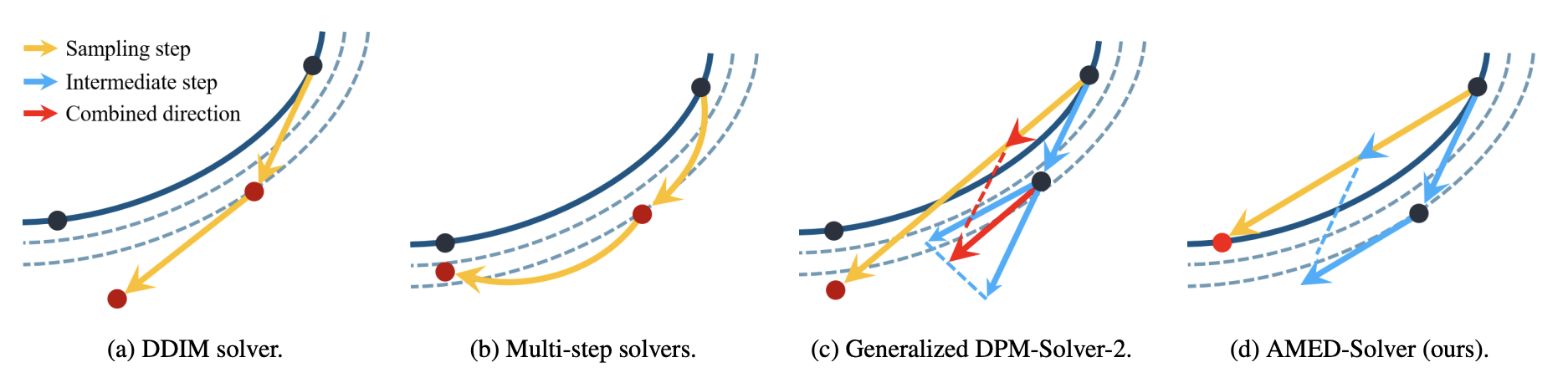 Illustration of several diffusion ODE solvers
First, we integrate both sides of equation $\eqref{eq:dm-ode}$, giving us the exact identity:
\begin{equation} \boldsymbol{x}_{t_{n+1}} - \boldsymbol{x}_{t_n} = \int_{t_n}^{t_{n+1}}\boldsymbol{v}_{\boldsymbol{\theta}}(\boldsymbol{x}_t, t)dt\end{equation}
If $\boldsymbol{v}$ were merely a one-dimensional scalar function, then by the "mean value theorem for integrals" we would know there exists a point $s_n\in(t_n, t_{n+1})$ such that
\begin{equation}\frac{1}{t_{n+1} - t_n}\int_{t_n}^{t_{n+1}}\boldsymbol{v}_{\boldsymbol{\theta}}(\boldsymbol{x}_t, t)dt = \boldsymbol{v}_{\boldsymbol{\theta}}(\boldsymbol{x}_{s_n}, s_n) \end{equation}
Unfortunately, the mean value theorem does not hold in general for vector-valued functions. Nevertheless, when $t_{n+1}-t_n$ is not too large, and under certain assumptions, we can still write down an analogous approximation:
\begin{equation}\frac{1}{t_{n+1} - t_n}\int_{t_n}^{t_{n+1}}\boldsymbol{v}_{\boldsymbol{\theta}}(\boldsymbol{x}_t, t)dt \approx \boldsymbol{v}_{\boldsymbol{\theta}}(\boldsymbol{x}_{s_n}, s_n) \end{equation}
which gives us
\begin{equation} \boldsymbol{x}_{t_n}\approx \boldsymbol{x}_{t_{n+1}} - \boldsymbol{v}_{\boldsymbol{\theta}}(\boldsymbol{x}_{s_n}, s_n)(t_{n+1}-t_n)\end{equation}
Of course, this is still only a formal solution—how to obtain $s_n$ and $\boldsymbol{x}_{s_n}$ remains an open question. For $\boldsymbol{x}_{s_n}$, we again use Euler's method as an estimate, i.e., $\tilde{\boldsymbol{x}}_{s_n}= \boldsymbol{x}_{t_{n+1}} - \boldsymbol{v}_{\boldsymbol{\theta}}(\boldsymbol{x}_{t_{n+1}}, t_{n+1})(t_{n+1} - s_n)$; for $s_n$, we instead use a small neural network to estimate it:
\begin{equation}s_n = g_{\boldsymbol{\phi}}(\boldsymbol{h}_{t_{n+1}}, t_{n+1})\end{equation}
where $\boldsymbol{\phi}$ are trainable parameters, and $\boldsymbol{h}_{t_{n+1}}$ are intermediate features of the U-Net model $\boldsymbol{v}_{\boldsymbol{\theta}}(\boldsymbol{x}_{t_{n+1}}, t_{n+1})$. Finally, to solve for the parameters $\boldsymbol{\phi}$, we adopt a distillation approach: we first use a solver with more steps to compute higher-precision trajectory point pairs $(\boldsymbol{x}_{t_n},\boldsymbol{x}_{t_{n+1}})$, and then minimize the estimation error. This is the AMED-Solver (Approximate MEan-Direction Solver) from the paper—it has the form of a regular ODE solver, but requires an additional distillation cost. That said, this distillation cost is nearly negligible compared to other distillation-based acceleration methods, which is why I think of it as a "custom-tailored" solver.
The word "custom-tailored" is key here. Research on accelerating diffusion ODE sampling has a long history, and thanks to the contributions of many researchers, training-free solvers have arguably already been pushed quite far—yet they still haven't been able to push the number of sampling steps down to the extreme. Barring some future breakthrough in our theoretical understanding of diffusion models, I don't think training-free solvers have much room left for significant improvement. So AMED's approach of adding a small amount of training cost to speed things up is both an unconventional detour and a natural, logical next step—"born of its time," so to speak.
Experimental Results
Before looking at the experimental results, let's first understand a concept called "NFE," short for "Number of Function Evaluations." Simply put, this is the number of times the model $\boldsymbol{v}_{\boldsymbol{\theta}}(\boldsymbol{x}_t, t)$ is executed, and it's directly tied to computational cost. For example, the first-order method has an NFE of 1 per iteration step, since it only needs to evaluate $\boldsymbol{v}_{\boldsymbol{\theta}}(\boldsymbol{x}_t, t)$ once, while the second-order method has an NFE of 2 per iteration step. The computational cost of $g_{\boldsymbol{\phi}}$ in AMED-Solver is tiny and can be ignored, so AMED-Solver's NFE per step is also counted as 2. To make a fair comparison, the total NFE across the entire sampling process needs to be held fixed when comparing different solvers.
The basic experimental results are shown in Table 2 of the original paper:
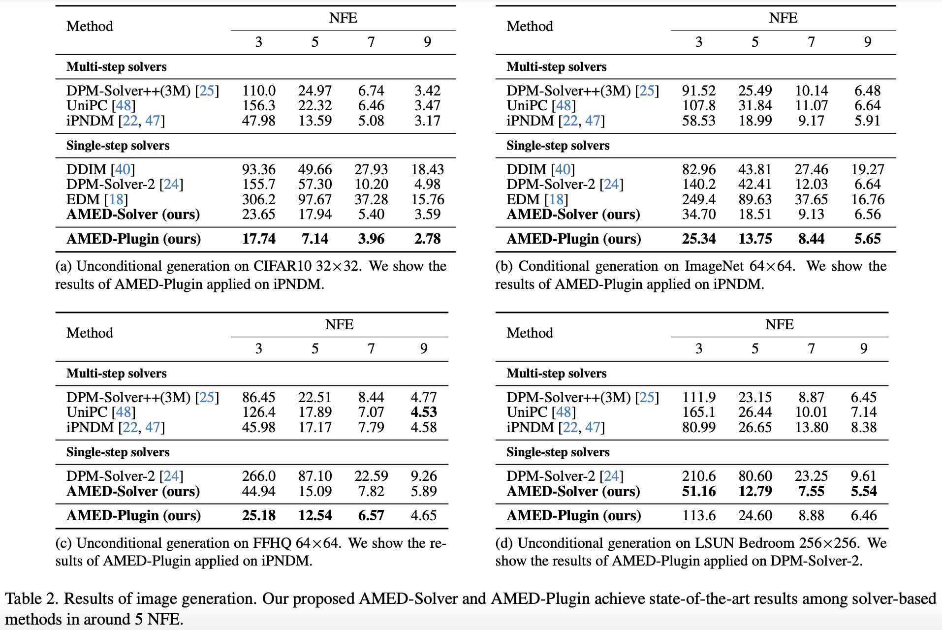 AMED experimental results (Table 2)
There are a few things in this table worth noting in particular. First, when the NFE is no more than 5, the second-order DPM-Solver and EDM actually perform worse than the first-order DDIM. This is because a solver's error depends not only on its order but also on the step size $t_{n+1}-t_n$, and roughly speaking the relationship is $\mathcal{O}((t_{n+1}-t_n)^m)$, where $m$ is the "order." When the total NFE is small, higher-order methods are forced to take larger steps, so the actual accuracy ends up worse, and performance suffers. Second, the also-second-order AMED-Solver achieves across-the-board SOTA at small NFEs, which nicely demonstrates the importance of being "custom-tailored." Third, "AMED-Plugin" here refers to a usage proposed in the original paper where AMED's idea is plugged into other ODE solvers; the details are more involved, but it achieves even better results.
Some readers might wonder: since each iteration step of a second-order method requires 2 NFEs, how can the table show odd NFE values? This is because the authors used a technique called "AFS (Analytical First Step)" to save one NFE. This technique comes from Genie: Higher-order denoising diffusion solvers, and specifically refers to the observation that, in the context of diffusion models, $\boldsymbol{v}_{\boldsymbol{\theta}}(\boldsymbol{x}_{t_N}, t_N)$ turns out to be very close to $\boldsymbol{x}_{t_N}$ (the exact behavior may differ somewhat across different diffusion models, but the core idea—that the first step can be solved analytically—is the same). So on the first sampling step, we directly substitute $\boldsymbol{x}_{t_N}$ for $\boldsymbol{v}_{\boldsymbol{\theta}}(\boldsymbol{x}_{t_N}, t_N)$, saving one NFE. Tables 8, 9, and 10 in the paper's appendix evaluate the effect of AFS on performance in more detail, for readers who are interested in digging further.
Finally, since AMED uses a distillation approach to train $g_{\boldsymbol{\phi}}$, some readers might wonder how it compares in performance to other distillation-based acceleration methods. Unfortunately, the paper doesn't provide such a comparison. I emailed the authors about this, and they told me that AMED's distillation cost is extremely low: for CIFAR-10, training takes less than 20 minutes on a single A100, and for 256-resolution images, only a few hours on 4 A100s—whereas other distillation-based acceleration approaches typically require days or even tens of days. That's why the authors regard AMED as work on solvers rather than as a distillation method. That said, the authors also mentioned that they hope to add a comparison against distillation-based methods when they get the chance.
Analysis of the Assumptions
Earlier, when discussing the generalization of the mean value theorem to vector-valued functions, we mentioned "under certain assumptions." So what exactly are these assumptions, and do they actually hold?
It isn't hard to construct counterexamples showing that even for two-dimensional functions, the mean value theorem for integrals doesn't hold in general—in other words, the mean value theorem for integrals only holds for one-dimensional functions. This means that if the integral mean value theorem were to hold for a high-dimensional function, the spatial trajectory described by that function could only be a straight line—that is, all the $\boldsymbol{x}_{t_0},\boldsymbol{x}_{t_1},\cdots,\boldsymbol{x}_{t_N}$ points along the sampling trajectory would have to lie on a single line. This is obviously a very strong assumption, and in practice it's almost certainly never exactly satisfied. But it also tells us something useful: for the integral mean value theorem to hold approximately in high-dimensional space, the sampling trajectory needs to stay as close as possible to some low-dimensional subspace.
To verify this, the paper's authors increased the number of sampling steps to obtain a more accurate sampling trajectory, and then performed principal component analysis on that trajectory. The results are shown below:
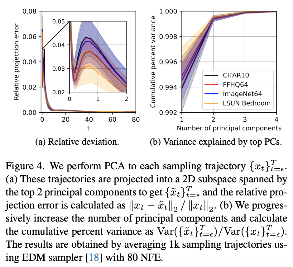 PCA of the diffusion ODE sampling trajectory
The PCA results show that keeping only the top-1 principal component already preserves most of the trajectory's accuracy, and keeping the top-2 principal components makes the remaining error nearly negligible. This tells us that the sampling trajectory is almost entirely concentrated within a two-dimensional subplane—indeed, it's very close to a straight line within that subplane. So when $t_{n+1}-t_n$ isn't too large, the integral mean value theorem in the diffusion model's high-dimensional space approximately holds after all.
This result might seem surprising at first, but on reflection it actually makes sense: in Diffusion Models Revisited (15): The General Recipe for Constructing an ODE (Part 2) and Diffusion Models Revisited (17): The General Recipe for Constructing an ODE (Part 3), we introduced the general procedure of first specifying a "pseudo-trajectory" from $\boldsymbol{x}_T$ to $\boldsymbol{x}_0$, and then constructing the corresponding diffusion ODE from that. In practice, the "pseudo-trajectories" we construct are always linear interpolations between $\boldsymbol{x}_T$ and $\boldsymbol{x}_0$ (possibly nonlinear in $t$, but linear in $\boldsymbol{x}_T$ and $\boldsymbol{x}_0$), so the constructed "pseudo-trajectories" are always straight lines. This in turn encourages the real diffusion trajectory to be close to a straight line as well, which explains the PCA results.
Summary
This post gave a brief overview of methods for accelerating diffusion ODE sampling, with particular focus on a newly released scheme called "AMED," published just a couple of days ago. This solver draws an analogy with the mean value theorem for integrals to construct its iteration scheme, and at an extremely low distillation cost, improves solver performance at low NFE.
Translated automatically with claude-sonnet-5; all equations are reproduced verbatim from the source. Copyright remains with the original author.