Generating Diffusion Models Chat (15): The General Procedure for Constructing ODEs (Part 2)

生成扩散模型漫谈（十五）：构建ODE的一般步骤（中） 苏剑林 · 2022-12-22 · Machine Learning differential equation generative model diffusion green's function

Last week I wrote Generating Diffusion Models Chat (14): The General Procedure for Constructing ODEs (Part 1) (at the time it didn't yet have the "Part 1" suffix), thinking I had already caught a glimpse of the general pattern for constructing ODE-based diffusion models. Not long after, however, @gaohuazuo, a brilliant commenter, gave a more efficient and intuitive scheme for constructing the Green's function, which left me feeling rather humbled. Recalling that this same reader had earlier given a wonderful description of the diffusion ODE in Generating Diffusion Models Chat (12): Tackling the Diffusion ODE Head-On (which indirectly inspired the results in the previous post), I really have to admire this person's insight.

After some discussion and reflection, I realized that the essence of this approach is the method of characteristics for first-order PDEs: by constructing a specific vector field, one guarantees the initial-value condition, and then by solving a differential equation, one guarantees the terminal-value condition — satisfying both conditions simultaneously, which really is a beautiful trick! Here, I've summarized what I learned into this post, as a follow-up to the previous one.

Recap

Let's briefly recap the results from the previous post. Suppose the random variable $\boldsymbol{x}_0\in\mathbb{R}^d$ is continuously transformed into $\boldsymbol{x}_T$, and this evolution follows the ODE

\begin{equation}\frac{d\boldsymbol{x}_t}{dt}=\boldsymbol{f}_t(\boldsymbol{x}_t)\label{eq-ode}\end{equation}

Then the corresponding distribution $p_t(\boldsymbol{x}_t)$ at time $t$ obeys the "continuity equation":

\begin{equation}\frac{\partial}{\partial t} p_t(\boldsymbol{x}_t) = - \nabla_{\boldsymbol{x}_t}\cdot\Big(\boldsymbol{f}_t(\boldsymbol{x}_t) p_t(\boldsymbol{x}_t)\Big)\label{eq:ode-f-eq-fp}\end{equation}

Writing $\boldsymbol{u}(t, \boldsymbol{x}_t)=(p_t( \boldsymbol{x}_t), \boldsymbol{f}_t(\boldsymbol{x}_t) p_t(\boldsymbol{x}_t))\in\mathbb{R}^{d+1}$, the continuity equation can be abbreviated as

\begin{equation}\left\{\begin{aligned} &\nabla_{(t,\, \boldsymbol{x}_t)}\cdot\boldsymbol{u}(t, \boldsymbol{x}_t)=0 \\ &\boldsymbol{u}_1(0, \boldsymbol{x}_0) = p_0(\boldsymbol{x}_0),\int \boldsymbol{u}_1(t, \boldsymbol{x}_t) d\boldsymbol{x}_t = 1 \end{aligned}\right.\label{eq:div-eq}\end{equation}

To solve this equation, we can use the idea of a Green's function, i.e., first solve

\begin{equation}\left\{\begin{aligned} &\nabla_{(t,\, \boldsymbol{x}_t)}\cdot\boldsymbol{G}(t, 0; \boldsymbol{x}_t, \boldsymbol{x}_0)=0\\ &\boldsymbol{G}_1(0, 0; \boldsymbol{x}_t, \boldsymbol{x}_0) = \delta(\boldsymbol{x}_t - \boldsymbol{x}_0),\int \boldsymbol{G}_1(t, 0; \boldsymbol{x}_t, \boldsymbol{x}_0) d\boldsymbol{x}_t = 1 \end{aligned}\right.\label{eq:div-green}\end{equation}

Then

\begin{equation}\boldsymbol{u}(t, \boldsymbol{x}_t) = \int \boldsymbol{G}(t, 0; \boldsymbol{x}_t, \boldsymbol{x}_0)p_0(\boldsymbol{x}_0) d\boldsymbol{x}_0 = \mathbb{E}_{\boldsymbol{x}_0\sim p_0(\boldsymbol{x}_0)}[\boldsymbol{G}(t, 0; \boldsymbol{x}_t, \boldsymbol{x}_0)]\label{eq:div-green-int}\end{equation}

is one of the solutions satisfying the constraints.

Geometric intuition

The idea behind a Green's function is actually quite simple: rather than rushing to tackle the generation of complex data, let's first assume that the data we want to generate consists of just a single point $\boldsymbol{x}_0$, and solve the generation problem for that single data point first. Some readers might think, isn't this trivial — just set $\boldsymbol{x}_T\times 0 + \boldsymbol{x}_0$ and be done with it? Of course it's not that simple, because what we need is a continuous, gradual generation process. As shown in the figure below, this means that every point $\boldsymbol{x}_T$ on $t=T$ at time $t=0$ travels along some smooth trajectory to reach $\boldsymbol{x}_0$:

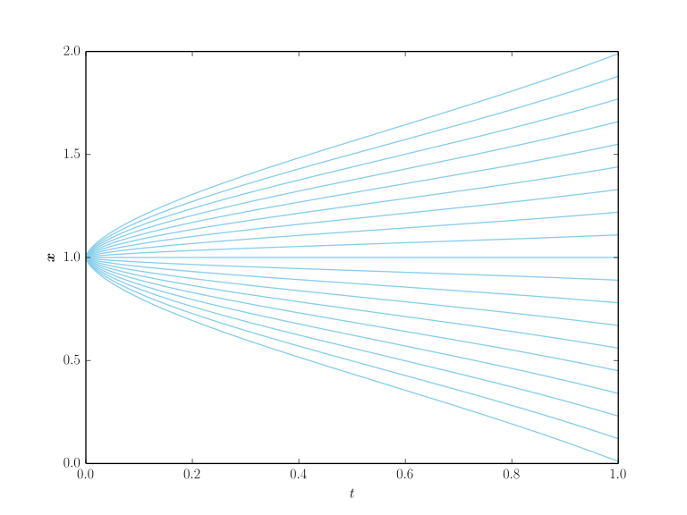Illustration of the Green's function. In the figure T=1; every point at t=1 travels along a specific trajectory to a point at t=0. Apart from the shared point, the trajectories do not overlap — these trajectories are the field lines of the Green's function

Our goal is simply to construct a generative model, so in principle we don't care what shape the trajectories take, as long as they all pass through $\boldsymbol{x}_0$. That means we're free to choose whatever family of trajectories we like that passes through $\boldsymbol{x}_0$, which we write as

\begin{equation}\boldsymbol{\varphi}_t(\boldsymbol{x}_t|\boldsymbol{x}_0) = \boldsymbol{x}_T\label{eq:track}\end{equation}

To emphasize again: this represents a family of trajectories starting at $\boldsymbol{x}_0$ and ending at $\boldsymbol{x}_T$, with independent and dependent variables $t,\boldsymbol{x}_t$ respectively. The starting point $\boldsymbol{x}_0$ is fixed, while the ending point $\boldsymbol{x}_T$ can vary arbitrarily; the shape of the trajectory doesn't matter — we could choose a straight line, a parabola, and so on.

Now let's differentiate both sides of equation $\eqref{eq:track}$. Since $\boldsymbol{x}_T$ can vary freely, it plays the role of an integration constant for the differential equation, so differentiating with respect to it just gives $\boldsymbol{0}$, and thus we have

\begin{equation}\frac{\partial \boldsymbol{\varphi}_t(\boldsymbol{x}_t|\boldsymbol{x}_0)}{\partial \boldsymbol{x}_t}\frac{d\boldsymbol{x}_t}{dt} + \frac{\partial \boldsymbol{\varphi}_t(\boldsymbol{x}_t|\boldsymbol{x}_0)}{\partial t} = \boldsymbol{0} \\ \Downarrow \\ \frac{d\boldsymbol{x}_t}{dt} = - \left(\frac{\partial \boldsymbol{\varphi}_t(\boldsymbol{x}_t|\boldsymbol{x}_0)}{\partial \boldsymbol{x}_t}\right)^{-1} \frac{\partial \boldsymbol{\varphi}_t(\boldsymbol{x}_t|\boldsymbol{x}_0)}{\partial t}\end{equation}

Comparing with equation $\eqref{eq-ode}$, we obtain

\begin{equation}\boldsymbol{f}_t(\boldsymbol{x}_t|\boldsymbol{x}_0) = - \left(\frac{\partial \boldsymbol{\varphi}_t(\boldsymbol{x}_t|\boldsymbol{x}_0)}{\partial \boldsymbol{x}_t}\right)^{-1} \frac{\partial \boldsymbol{\varphi}_t(\boldsymbol{x}_t|\boldsymbol{x}_0)}{\partial t}\label{eq:f-xt-x0}\end{equation}

Here we've replaced the original notation $\boldsymbol{f}_t(\boldsymbol{x}_t)$ with $\boldsymbol{f}_t(\boldsymbol{x}_t|\boldsymbol{x}_0)$, to indicate that the trajectories share the common point $\boldsymbol{x}_0$. In other words, the ODE trajectories corresponding to the force field $\boldsymbol{f}_t(\boldsymbol{x}_t|\boldsymbol{x}_0)$ constructed this way must pass through $\boldsymbol{x}_0$ — which guarantees the initial-value condition for the Green's function.

The method of characteristics

Since the initial-value condition is now guaranteed, we might as well ask for a bit more: let's also guarantee the terminal-value condition. The terminal-value condition means that we want the distribution of $\boldsymbol{x}_T$ at time $t=T$ to be a simple distribution independent of $\boldsymbol{x}_0$. The main drawback of the solution framework in the previous post was that it couldn't directly guarantee the simplicity of the terminal distribution — this could only be examined after the fact through analysis. The approach in this post, by contrast, first designs a specific $\boldsymbol{f}_t(\boldsymbol{x}_t|\boldsymbol{x}_0)$ to guarantee the initial-value condition, leaving us the remaining freedom to guarantee the terminal-value condition. Moreover, once both the initial and terminal conditions are simultaneously satisfied, the integral condition is automatically satisfied as well, given that the continuity equation $\eqref{eq:ode-f-eq-fp}$ holds.

In mathematical terms, what we want is: given $\boldsymbol{f}_t(\boldsymbol{x}_t|\boldsymbol{x}_0)$ and $p_T(\boldsymbol{x}_T)$, solve the equation $\eqref{eq:ode-f-eq-fp}$. This is a first-order PDE, which can be solved using the "method of characteristics" — for background theory, see my earlier post The Method of Characteristics for First-Order PDEs. First, let's rewrite equation $\eqref{eq:ode-f-eq-fp}$ equivalently as

\begin{equation}\frac{\partial}{\partial t} p_t(\boldsymbol{x}_t|\boldsymbol{x}_0) + \nabla_{\boldsymbol{x}_t}p_t(\boldsymbol{x}_t|\boldsymbol{x}_0) \cdot \boldsymbol{f}_t(\boldsymbol{x}_t|\boldsymbol{x}_0) = - p_t(\boldsymbol{x}_t|\boldsymbol{x}_0) \nabla_{\boldsymbol{x}_t}\cdot \boldsymbol{f}_t(\boldsymbol{x}_t|\boldsymbol{x}_0)\end{equation}

As before, since we're now solving for a given starting point $\boldsymbol{x}_0$, in the equation above we've replaced $p_t(\boldsymbol{x}_t)$ with $p_t(\boldsymbol{x}_t|\boldsymbol{x}_0)$, to indicate that this is the solution starting from $\boldsymbol{x}_0$.

The idea behind the method of characteristics is to first consider the solution of the PDE along a particular trajectory, which converts the partial differential equation into an ordinary differential equation, reducing the difficulty of solving it. Specifically, suppose $\boldsymbol{x}_t$ is a function of $t$, and we solve it along the trajectory of equation $\eqref{eq-ode}$. Since equation $\eqref{eq-ode}$ holds, once we replace $\boldsymbol{f}_t(\boldsymbol{x}_t|\boldsymbol{x}_0)$ on the left-hand side of the equation above with $\frac{d\boldsymbol{x}_t}{dt}$, the left-hand side turns out to be exactly the total derivative of $p_t(\boldsymbol{x}_t|\boldsymbol{x}_0)$, so we then have

\begin{equation}\frac{d}{dt}p_t(\boldsymbol{x}_t|\boldsymbol{x}_0) = - p_t(\boldsymbol{x}_t|\boldsymbol{x}_0) \nabla_{\boldsymbol{x}_t}\cdot \boldsymbol{f}_t(\boldsymbol{x}_t|\boldsymbol{x}_0)\end{equation}

Note that here all instances of $\boldsymbol{x}_t$ should be replaced by their corresponding functions of $t$, which in principle can be solved for from the trajectory equation $\eqref{eq:track}$. After this substitution, both $p$ and $\boldsymbol{f}$ on the right are purely functions of $t$, so the equation above is simply a linear ordinary differential equation in $p$, which can be solved to give

\begin{equation}p_t(\boldsymbol{x}_t|\boldsymbol{x}_0) = C \exp\left(\int_t^T \nabla_{\boldsymbol{x}_s}\cdot \boldsymbol{f}_s(\boldsymbol{x}_s|\boldsymbol{x}_0) ds\right)\end{equation}

Substituting the terminal condition $p_T(\boldsymbol{x}_T)$, we obtain $C=p_T(\boldsymbol{x}_T)$, i.e.,

\begin{equation}p_t(\boldsymbol{x}_t|\boldsymbol{x}_0) = p_T(\boldsymbol{x}_T) \exp\left(\int_t^T \nabla_{\boldsymbol{x}_s}\cdot \boldsymbol{f}_s(\boldsymbol{x}_s|\boldsymbol{x}_0) ds\right)\label{eq:pt-xt-x0}\end{equation}

Substituting $\boldsymbol{x}_T$ from the trajectory equation $\eqref{eq:track}$, we get a function purely of $t,\boldsymbol{x}_t,\boldsymbol{x}_0$, which is precisely the Green's function $\boldsymbol{G}_1(t, 0; \boldsymbol{x}_t, \boldsymbol{x}_0)$ we set out to find, and correspondingly $\boldsymbol{G}_{> 1}(t, 0; \boldsymbol{x}_t, \boldsymbol{x}_0)=p_t(\boldsymbol{x}_t|\boldsymbol{x}_0) \boldsymbol{f}_t(\boldsymbol{x}_t|\boldsymbol{x}_0)$.

Training objective

With the Green's function in hand, we can obtain

\begin{equation}\begin{aligned} \boldsymbol{u}_1(t, \boldsymbol{x}_t) =&\, \int p_t(\boldsymbol{x}_t|\boldsymbol{x}_0) p_0(\boldsymbol{x}_0) d\boldsymbol{x}_0 = p_t(\boldsymbol{x}_t)\\ \boldsymbol{u}_{> 1}(t, \boldsymbol{x}_t) =&\, \int \boldsymbol{f}_t(\boldsymbol{x}_t|\boldsymbol{x}_0) p_t(\boldsymbol{x}_t|\boldsymbol{x}_0) p_0(\boldsymbol{x}_0) d\boldsymbol{x}_0 \end{aligned}\end{equation}

and thus

\begin{equation}\begin{aligned} \boldsymbol{f}_t(\boldsymbol{x}_t)=&\,\frac{\boldsymbol{u}_{> 1}(t, \boldsymbol{x}_t)}{\boldsymbol{u}_1(t, \boldsymbol{x}_t)} \\ =&\,\int \boldsymbol{f}_t(\boldsymbol{x}_t|\boldsymbol{x}_0) \frac{p_t(\boldsymbol{x}_t|\boldsymbol{x}_0) p_0(\boldsymbol{x}_0)}{p_t(\boldsymbol{x}_t)} d\boldsymbol{x}_0 \\ =&\,\int \boldsymbol{f}_t(\boldsymbol{x}_t|\boldsymbol{x}_0) p_t(\boldsymbol{x}_0|\boldsymbol{x}_t) d\boldsymbol{x}_0 \\ =&\,\mathbb{E}_{\boldsymbol{x}_0\sim p_t(\boldsymbol{x}_0|\boldsymbol{x}_t)}\left[\boldsymbol{f}_t(\boldsymbol{x}_t|\boldsymbol{x}_0)\right] \end{aligned}\end{equation}

Following the method for constructing score-matching objectives described in Generating Diffusion Models Chat (5): The General SDE Framework, we can construct the training objective

\begin{equation}\begin{aligned}&\,\mathbb{E}_{\boldsymbol{x}_t\sim p _t(\boldsymbol{x}_t)}\Big[\mathbb{E}_{\boldsymbol{x}_0\sim p _t(\boldsymbol{x}_0|\boldsymbol{x}_t)}\left[\left\Vert \boldsymbol{v}_{\boldsymbol{\theta}}(\boldsymbol{x}_t, t) - \boldsymbol{f}_t(\boldsymbol{x}_t|\boldsymbol{x}_0)\right\Vert^2\right]\Big] d\boldsymbol{x}_t \\ =&\, \mathbb{E}_{\boldsymbol{x}_0,\boldsymbol{x}_t \sim p_t(\boldsymbol{x}_t|\boldsymbol{x}_0)p _0(\boldsymbol{x}_0)}\left[\left\Vert \boldsymbol{v}_{\boldsymbol{\theta}}(\boldsymbol{x}_t, t) - \boldsymbol{f}_t(\boldsymbol{x}_t|\boldsymbol{x}_0)\right\Vert^2\right] \end{aligned}\label{eq:score-match}\end{equation}

which is formally identical to the "Conditional Flow Matching" formulation given in Flow Matching for Generative Modeling. Later on we'll also see that all of that paper's results can be derived from the approach in this post. Once training is complete, we can generate samples by solving equation $\frac{d\boldsymbol{x}_t}{dt}=\boldsymbol{v}_{\boldsymbol{\theta}}(\boldsymbol{x}_t, t)$. From this training objective, it's also clear that the only requirement on $p_t(\boldsymbol{x}_t|\boldsymbol{x}_0)$ is that it be easy to sample from.

Some examples

Perhaps the abstract results above are still not very easy to grasp, so let's now go through some concrete examples to help build intuition for this framework. As for the method of characteristics itself, as I mentioned in The Method of Characteristics for First-Order PDEs, I too initially found it to feel like sleight of hand — following the steps isn't hard, but somehow one never quite grasps the essence of it. Understanding it requires repeated careful thought, which I can't do on the reader's behalf.

Straight-line trajectories

As the simplest example, suppose $\boldsymbol{x}_T$ transforms into $\boldsymbol{x}_0$ along a straight-line trajectory. For simplicity we can also set $T$ to 1 without loss of generality, so the equation for $\boldsymbol{x}_t$ can be written as

\begin{equation}\boldsymbol{x}_t = (\boldsymbol{x}_1 - \boldsymbol{x}_0)t + \boldsymbol{x}_0\quad\Rightarrow\quad \frac{\boldsymbol{x}_t - \boldsymbol{x}_0}{t} + \boldsymbol{x}_0 = \boldsymbol{x}_1\label{eq:simplest-x1}\end{equation}

According to equation $\eqref{eq:f-xt-x0}$, we have

\begin{equation}\boldsymbol{f}_t(\boldsymbol{x}_t|\boldsymbol{x}_0) = \frac{\boldsymbol{x}_t - \boldsymbol{x}_0}{t}\end{equation}

Here $\nabla_{\boldsymbol{x}_t}\cdot \boldsymbol{f}_t(\boldsymbol{x}_t|\boldsymbol{x}_0)=\frac{d}{t}$, so according to equation $\eqref{eq:pt-xt-x0}$ we have

\begin{equation}p_t(\boldsymbol{x}_t|\boldsymbol{x}_0) = \frac{p_1(\boldsymbol{x}_1)}{t^d}\end{equation}

Substituting into $\boldsymbol{x}_1$ in equation $\eqref{eq:simplest-x1}$, we obtain

\begin{equation}p_t(\boldsymbol{x}_t|\boldsymbol{x}_0) = \frac{p_1\left(\frac{\boldsymbol{x}_t - \boldsymbol{x}_0}{t} + \boldsymbol{x}_0\right)}{t^d}\end{equation}

In particular, if $p_1(\boldsymbol{x}_1)$ is the standard normal distribution, then the equation above in effect means $p_t(\boldsymbol{x}_t|\boldsymbol{x}_0)=\mathcal{N}(\boldsymbol{x}_t;(1-t)\boldsymbol{x}_0,t^2\boldsymbol{I})$, which is precisely one of the familiar Gaussian diffusion models. The new result offered by this framework is that it allows us to choose a more general prior distribution $p_1(\boldsymbol{x}_1)$, such as a uniform distribution. Furthermore, as already mentioned when introducing score matching $\eqref{eq:score-match}$, all we need to know about $p_t(\boldsymbol{x}_t|\boldsymbol{x}_0)$ is how to sample from it, and the equation above tells us that all we need is for the prior distribution to be easy to sample from, because:

\begin{equation}\boldsymbol{x}_t\sim p_t(\boldsymbol{x}_t|\boldsymbol{x}_0)\quad\Leftrightarrow\quad \boldsymbol{x}_t=(1-t)\boldsymbol{x}_0 + t\boldsymbol{\varepsilon},\,\boldsymbol{\varepsilon}\sim p_1(\boldsymbol{\varepsilon})\end{equation}

Demonstration

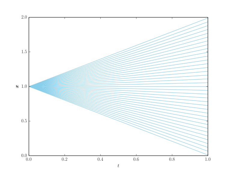
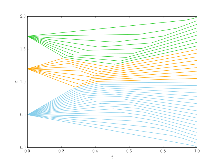
Note that our assumption that the trajectory from $\boldsymbol{x}_0$ to $\boldsymbol{x}_1$ is a straight line applies only to single-point generation, i.e., to the Green's function solution. Once we superpose the Green's functions to obtain the force field $\boldsymbol{f}_t(\boldsymbol{x}_t)$ corresponding to a general distribution, the resulting generation trajectories are no longer straight lines.

The figure below illustrates the trajectories for multi-point generation when the prior distribution is uniform:

Single-point generationTwo-point generationThree-point generation

Reference plotting code:

import numpy as np
from scipy.integrate import odeint
import matplotlib
import matplotlib.pyplot as plt
matplotlib.rc('text', usetex=True)
matplotlib.rcParams['text.latex.preamble']=[r"\usepackage{amsmath}"]

prior = lambda x: 0.5 if 2 >= x >= 0 else 0
p = lambda xt, x0, t: prior((xt - x0) / t + x0) / t
f = lambda xt, x0, t: (xt - x0) / t

def f_full(xt, t):
    x0s = [0.5, 0.5, 1.2, 1.7]  # 0.5出现两次，代表其频率是其余的两倍
    fs = np.array([f(xt, x0, t) for x0 in x0s]).reshape(-1)
    ps = np.array([p(xt, x0, t) for x0 in x0s]).reshape(-1)
    return (fs * ps).sum() / (ps.sum() + 1e-8)

for x1 in np.arange(0.01, 1.99, 0.10999/2):
    ts = np.arange(1, 0, -0.001)
    xs = odeint(f_full, x1, ts).reshape(-1)[::-1]
    ts = ts[::-1]
    if abs(xs[0] - 0.5) < 0.1:
        _ = plt.plot(ts, xs, color='skyblue')
    elif abs(xs[0] - 1.2) < 0.1:
        _ = plt.plot(ts, xs, color='orange')
    else:
        _ = plt.plot(ts, xs, color='limegreen')

plt.xlabel('$t$')
plt.ylabel(r'$\boldsymbol{x}$')
plt.show()

General extension

In fact, the result above can be generalized further to

\begin{equation}\boldsymbol{x}_t = \boldsymbol{\mu}_t(\boldsymbol{x}_0) + \sigma_t \boldsymbol{x}_1\quad\Rightarrow\quad \frac{\boldsymbol{x}_t - \boldsymbol{\mu}_t(\boldsymbol{x}_0)}{\sigma_t }= \boldsymbol{x}_1\end{equation}

Here $\boldsymbol{\mu}_t(\boldsymbol{x}_0)$ is any $\mathbb{R}^d\mapsto\mathbb{R}^d$ function satisfying $\boldsymbol{\mu}_0(\boldsymbol{x}_0)=\boldsymbol{x}_0, \boldsymbol{\mu}_1(\boldsymbol{x}_0)=\boldsymbol{0}$, and $\sigma_t$ is any monotonically increasing function satisfying $\sigma_0=0,\sigma_1=1$. According to equation $\eqref{eq:f-xt-x0}$, we have

\begin{equation}\boldsymbol{f}_t(\boldsymbol{x}_t|\boldsymbol{x}_0) = \dot{\boldsymbol{\mu}}_t(\boldsymbol{x}_0) + \frac{\dot{\sigma}_t}{\sigma_t}(\boldsymbol{x}_t - \boldsymbol{\mu}_t(\boldsymbol{x}_0))\end{equation}

This is also equivalent to equation $(15)$ in Flow Matching for Generative Modeling. Here $\nabla_{\boldsymbol{x}_t}\cdot \boldsymbol{f}_t(\boldsymbol{x}_t|\boldsymbol{x}_0)=\frac{d\dot{\sigma}_t}{\sigma_t}$, so according to equation $\eqref{eq:pt-xt-x0}$ we have

\begin{equation}p_t(\boldsymbol{x}_t|\boldsymbol{x}_0) = \frac{p_1(\boldsymbol{x}_1)}{\sigma_t^d}\end{equation}

Substituting into $\boldsymbol{x}_1$, the final result is

\begin{equation}p_t(\boldsymbol{x}_t|\boldsymbol{x}_0) = \frac{p_1\left(\frac{\boldsymbol{x}_t - \boldsymbol{\mu}_t(\boldsymbol{x}_0)}{\sigma_t }\right)}{\sigma_t^d}\end{equation}

This is the general result for linear ODE diffusion, encompassing Gaussian diffusion while also allowing non-Gaussian prior distributions.

Getting more complex?

In all the examples above, the trajectory of $\boldsymbol{x}_t$ is constructed via a simple linear interpolation between (some transformation of) $\boldsymbol{x}_0$ and $\boldsymbol{x}_1$, where the interpolation weight is purely a function of $t$. A natural question then arises: could we consider more complex trajectories? In principle, yes — but greater complexity implies more hidden assumptions, and it's usually very hard to check whether the target data actually supports those assumptions. So in practice, more complex trajectories are generally not considered. Moreover, for more complex trajectories, analytical solutions tend to be harder to obtain, making both theoretical analysis and experiments difficult to carry out.

More importantly, the trajectories we've been assuming so far are just trajectories for single-point generation. As already demonstrated, even when we assume straight lines, multi-point generation still produces complex curves. So if we make even the single-point generation trajectories unnecessarily complex, we can imagine that the complexity of the multi-point generation trajectories would become extremely high, and the model could become highly unstable.

Summary

Continuing from the previous post, this article once again discusses ideas for constructing ODE-based diffusion models. This time we started from geometric intuition: by constructing a specific vector field, we guarantee that the result satisfies the initial-value distribution condition, and then by solving a differential equation, we guarantee the terminal-value distribution condition, obtaining a Green's function that satisfies both the initial- and terminal-value conditions simultaneously. In particular, this method allows us to use an arbitrary simple distribution as the prior, freeing us from the traditional reliance on the Gaussian distribution when constructing diffusion models.