Attention's Scale Factor from the Perspective of Gradient Maximization

从梯度最大化看Attention的Scale操作苏剑林 · 2023-10-22 · Machine Learning optimization gradient attention

We know that the Scale factor in Scaled Dot-Product Attention is $\frac{1}{\sqrt{d}}$, where $d$ is the dimension of $\boldsymbol{q},\boldsymbol{k}$. The usual explanation for this Scale factor is: if we don't divide by $\sqrt{d}$, then the initial Attention distribution would be very close to a one-hot distribution, which would cause vanishing gradients and make the model impossible to train. However, it can be shown that when the Scale equals 0, we also run into vanishing gradients — in other words, the Scale being either too large or too small is problematic.

So how large should the Scale be? Is $\frac{1}{\sqrt{d}}$ actually the optimal choice? This post attempts to answer this question from the perspective of gradients.

Existing Results

In A Brief Discussion on Transformer Initialization, Parameterization, and Normalization, we already derived the standard Scale factor $\frac{1}{\sqrt{d}}$. The idea behind that derivation is simple: assuming that at initialization $\boldsymbol{q},\boldsymbol{k}\in\mathbb{R}^d$ are all sampled from a distribution with "mean 0, variance 1", we can compute

\begin{equation}\mathbb{V}ar[\boldsymbol{q}\cdot\boldsymbol{k}] = d\end{equation}more

and so we divide $\boldsymbol{q}\cdot\boldsymbol{k}$ by $\sqrt{d}$, making the variance of the Attention Score equal to 1. In other words, the earlier derivation was based purely on the belief that "mean 0, variance 1" would be better, without any explanation of why setting the Attention Score's variance to 1 would actually help, nor any evaluation of whether $\frac{1}{\sqrt{d}}$ genuinely solves the vanishing-gradient problem.

Of course, existing experiments do show that $\frac{1}{\sqrt{d}}$ alleviates this problem, at least to some extent — but that's still just an empirical observation. We'd like to know, in theory, exactly how much "to some extent" really means.

Computing the Gradient

Since gradients are involved, the best approach is simply to compute the gradient directly and then define an optimization objective. Let $p_i = e^{\alpha s_i}/Z$, $i \in \{1,2,...,n\}$, and let $Z=\sum_i e^{\alpha s_i}$ be the normalization factor. Then we can directly compute:

\begin{equation}\frac{\partial p_i}{\partial s_j} = \left\{\begin{aligned} \alpha(p_i - p_i^2),&\quad i=j\\ -\alpha p_i p_j,&\quad i\neq j \end{aligned}\right.\end{equation}

or more compactly, $\partial p_i/\partial s_j = \alpha(p_i\delta_{i,j} - p_i p_j)$. Clearly, when $\alpha\to 0$, the gradient is 0; and when $\alpha\to\infty$, only one entry of $p_i$ is 1 and the rest are 0 (assuming $s_i$ has a unique maximum), so the gradient is also 0.

To make optimization easier, we should choose $\alpha$ so as to maximize the gradient as much as possible. To this end, we use the L1 norm as a measure of gradient magnitude:

\begin{equation}\frac{1}{2}\left\Vert\frac{\partial p}{\partial s}\right\Vert_1=\frac{1}{2}\sum_{i,j}\left|\frac{\partial p_i}{\partial s_j}\right|=\frac{1}{2}\sum_i \alpha(p_i - p_i^2) + \frac{1}{2}\sum_{i\neq j} \alpha p_i p_j = \alpha\left(1 - \sum_i p_i^2\right)\label{eq:target}\end{equation}

It's not hard to guess from the final result that the reason we chose the L1 norm rather than some other norm is simply that it gives a sufficiently simple result. It's worth pointing out that $\sum_i p_i^2$ appears here, which is essentially the "Rényi entropy" we introduced in How to Measure the Sparsity of Data?. Like Shannon entropy, it is also a measure of uncertainty.

With this optimization objective in hand, we can proceed to maximize it. Note that the definition of $p_i$ also involves $\alpha$, so this is a complicated nonlinear objective in terms of $\alpha$, and finding an analytical solution appears hopeless. However, we can find approximate solutions for some special cases.

Normal Distribution

First, let's continue from the previous result: once we've made the Attention Score have mean 0 and variance 1 by dividing by $\sqrt{d}$, we can approximately assume $s_i\sim\mathcal{N}(0,1)$, and then find the optimal solution for $\alpha$. If $\alpha=1$, this means that the original $\frac{1}{\sqrt{d}}$ was already the optimal Scale ratio; otherwise, $\frac{\alpha}{\sqrt{d}}$ is the best Scale ratio.

We estimate the sum using an expectation

\begin{equation}\sum_i p_i^2 = \frac{\sum_i e^{2\alpha s_i}}{\left(\sum_i e^{\alpha s_i}\right)^2} = \frac{\frac{1}{n}\sum_i e^{2\alpha s_i}}{n\left(\frac{1}{n}\sum_i e^{\alpha s_i}\right)^2} \approx \frac{\mathbb{E}_s[e^{2\alpha s}]}{n\left(\mathbb{E}_s[e^{\alpha s}]\right)^2}\label{eq:approx}\end{equation}

For $s$ following a standard normal distribution, we have

\begin{equation}\mathbb{E}_s[e^{\alpha s}] = \int \frac{1}{\sqrt{2\pi}}e^{-s^2/2}e^{\alpha s} ds = e^{\alpha^2 / 2}\label{eq:normal}\end{equation}

Substituting this into the equation above, and then into equation $\eqref{eq:target}$, we get

\begin{equation}\alpha\left(1 - \sum_i p_i^2\right)\approx\alpha\left(1 - \frac{e^{\alpha^2}}{n}\right)\end{equation}

Although this final approximation is already quite simplified, it's still not easy to find its maximum analytically. That's fine, though — we can sweep over a range of values of $n$ and numerically solve for the $\alpha^*$ that maximizes it, which lets us see roughly how $\alpha^*$ relates to $n$. The reference Mathematica code is as follows:

(*定义函数*)
f[a_, n_] := a*(1 - Exp[a^2]/n)
(*找到函数的最大点对应的a*)
FindArg[n_] := 
 Module[{a}, a = a /. Last@NMaximize[{f[a, n], a > 0}, a][[2]]; a]
(*给定n的范围*)
nRange = 40*Range[1, 500];
(*求出每个n对应的a*)
args = FindArg /@ nRange;
(*画出a与n的函数图像*)
ListLinePlot[{args, 0.84*Log[nRange]^0.5}, 
 DataRange -> {40, 20000}, AxesLabel -> {"n", "a"}, 
 PlotLegends -> {Row[{"a", Superscript["", "*"]}], 
   TraditionalForm[HoldForm[0.84*Sqrt[Log[n]]]]}]

After fitting, I found that within a certain range, the optimal point $\alpha^*$ and $n$ roughly satisfy the relationship $\alpha\approx 0.84\sqrt{\log n}$, so I've also plotted the corresponding approximate function alongside it:

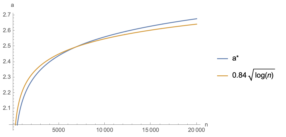Relationship between optimal alpha and n for the standard normal distribution

As we can see, over a fairly wide range, the optimal value of $\alpha^*$ lies between $2\sim 3$. So, as a compromise, blindly taking $\frac{2.5}{\sqrt{d}}$ as Attention's Scale factor is theoretically more favorable for optimization.

Cosine Distribution

Now let's consider another, less common example: when we normalize all the $\boldsymbol{q},\boldsymbol{k}$ using $l_2$ normalization to turn them into unit vectors, their inner products become the cosine of the angle between them, i.e., $s_i$ approximately follows the distribution of the cosine of the angle between two random vectors in $d$-dimensional space. This distribution may be unfamiliar to some readers, but we've discussed it before in The Distribution of the Angle Between Two Random Vectors in n-Dimensional Space. Its probability density has the form

\begin{equation}p(s)\propto (1-s^2)^{(d-3)/2}\end{equation}

This doesn't look too complicated, but in fact it's much harder to handle than the normal distribution, mainly because $\mathbb{E}_s[e^{\alpha s}]$ can no longer be expressed in terms of elementary functions the way it could in equation $\eqref{eq:normal}$. That said, it's not a problem for Mathematica to solve numerically. Following the same approach as in the previous section, the approximation in equation $\eqref{eq:approx}$ still applies: we first numerically solve for the maximum, then fit the results, which are shown below (in the figure, $d=128$, and $\alpha^*$ is related to $d$):

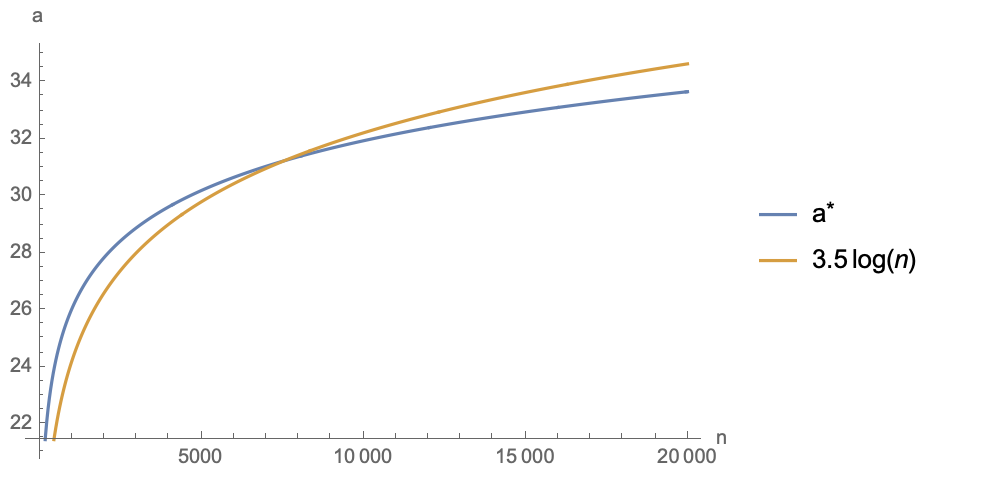Relationship between optimal alpha and n for the cosine distribution

As we can see, $\alpha^*$ and $3.5\log n$ fit each other quite well too (for a different $d$, the coefficient $3.5$ would change). We can also see that over a fairly wide range, $\alpha^*$ falls between $25\sim 35$. So if we were to use the $\cos$ value as the Attention Score, we would need to multiply it by a Scale between $25\sim 35$ in order for the model to be reasonably trainable. This also explains why, when constructing a Softmax distribution using $\cos$ values (as in AM-Softmax or SimCSE), we need to multiply by a Scale of around 30 after $\cos$ — because without doing so, the model is very hard to train.

For different values of $d$ and $n$, readers are welcome to modify the following code themselves to compute the optimal $\alpha$:

(*定义函数*)
h[a_] := 
 Integrate[Exp[a*s]*(1 - s^2)^((d - 3)/2), {s, -1, 1}, 
  Assumptions -> {d > 10}]
g[a_] = h[a]/h[0] // FullSimplify;
f[a_, n_] := a (1 - g[2*a]/g[a]^2/n) /. {d -> 128}
(*找到函数的最大点对应的a*)
FindArg[n_] := 
 Module[{a}, a = a /. Last@NMaximize[{f[a, n], a > 0}, a][[2]]; a]
(*给定n的范围*)
nRange = 40*Range[1, 500];
(*求出每个n对应的a*)
args = FindArg /@ nRange;
(*画出a与n的函数图像*)
ListLinePlot[{args, 3.5*Log[nRange]}, 
 DataRange -> {40, 20000}, AxesLabel -> {"n", "a"}, 
 PlotLegends -> {Row[{"a", Superscript["", "*"]}], 
   TraditionalForm[HoldForm[3.5*Log[n]]]}]

The title and results of this post — especially the finding in the cosine distribution case that $\alpha$ is approximately proportional to $\log n$ — naturally bring to mind another article discussing Attention's Scale operation: Attention's Scale Operation Viewed Through Entropy Invariance. Indeed, there is a real connection between the two posts. The optimization objective $\eqref{eq:target}$ in this post involves the "Rényi entropy", while the entropy in "entropy invariance" refers to Shannon information entropy — and the properties of the two are, to a large extent, consistent with each other. Maximizing equation $\eqref{eq:target}$ pushes it into a "slowly varying" region, which means that the "Rényi entropy" changes very slowly with respect to $n$, and correspondingly that the Shannon entropy also changes very slowly with respect to $n$ — which is roughly equivalent to entropy invariance.

Furthermore, for bidirectional attention (Encoder), assuming the training samples all have the same length, $n$ is a constant, so we can compute the corresponding optimal $\alpha$ from $n$ and simply fix it in the model. But for unidirectional attention (Decoder), the value of $n$ actually differs for each token (the position id increases by 1 each time), so in theory it's impossible to maximize equation $\eqref{eq:target}$ simultaneously for every token. However, since $\alpha^*$ changes slowly with respect to $n$, we can just pick a roughly suitable value — for instance, $n=L_{\max} / 2$ — which would give reasonably friendly gradients for most tokens.

Summary

This post examined the choice of Attention's Scale factor from the perspective of gradients. As is well known, the "standard answer" for this Scale factor is $\frac{1}{\sqrt{d}}$, but its derivation never actually addressed the question of its optimality. So here I defined an optimization objective based on the Softmax gradient, and explored the optimal value of the Scale factor from the standpoint of maximizing that objective. These results can be used both to improve Attention's Scale factor and to explain the temperature parameter used in contrastive learning with $\cos$ similarity.