Is SimCSE Still SOTA for Chinese Tasks? Some Supplementary Experiments
Earlier this year, inspired by BERT-flow, I came up with a method called "BERT-whitening," which for a while became the new SOTA for semantic similarity (see You Probably Don't Need BERT-flow: A Linear Transformation Rivaling BERT-flow, based on the paper Whitening Sentence Representations for Better Semantics and Faster Retrieval). However, this "good times" didn't last long — shortly after BERT-whitening was posted to Arxiv, at least two new papers appeared there with results clearly superior to BERT-whitening's.
The first is Generating Datasets with Pretrained Language Models, which uses templates to unsupervisedly construct data pairs from GPT2_XL to train a similarity model. Personally I find it somewhat inspiring and the results decent, but the cost and variance of reproducing it are too large. The other is the protagonist of this post, SimCSE: Simple Contrastive Learning of Sentence Embeddings, whose proposed SimCSE significantly outperforms BERT-flow and BERT-whitening on English data, and the method is remarkably simple.
So, does SimCSE work equally well on Chinese? Can it substantially boost the performance of Chinese semantic similarity? This post presents some supplementary experiments on that question.
Open-source code: https://github.com/bojone/SimCSE
SimCSE
First, a brief introduction to SimCSE. In fact, SimCSE can be seen as a simplified version of SimBERT (for SimBERT, see Having Your Cake and Eating It Too: The SimBERT Model that Combines Retrieval and Generation). The simplifications are as follows:
1. SimCSE removes SimBERT's generation component, keeping only the retrieval model;
2. Since SimCSE has no labeled data, each sentence is treated as its own similar sentence when fed into the model.
Put simply, this essentially trains a contrastive learning model using (self, self) as positive pairs and (self, others) as negative pairs. Of course, in practice it's not quite that simple — if the two positive samples are exactly identical, generalization suffers considerably. Generally speaking, we would use some data augmentation technique to introduce a bit of difference between the two positive samples, but how to do data augmentation in NLP is itself a tricky problem. SimCSE proposes an extremely simple solution: just use Dropout as the data augmentation!
Specifically, $N$ sentences pass through an Encoder with Dropout to get vectors $\boldsymbol{h}^{(0)}_1,\boldsymbol{h}^{(0)}_2,\cdots,\boldsymbol{h}^{(0)}_N$, and then this same batch of sentences is passed through the Encoder again (this time with a different random Dropout) to get vectors $\boldsymbol{h}^{(1)}_1,\boldsymbol{h}^{(1)}_2,\cdots,\boldsymbol{h}^{(1)}_N$. We can treat $(\boldsymbol{h}^{(0)}_i,\boldsymbol{h}^{(1)}_i)$ as a (slightly different) positive pair, giving the training objective:
\begin{equation}-\sum_{i=1}^N\sum_{\alpha=0,1}\log \frac{e^{\cos(\boldsymbol{h}^{(\alpha)}_i, \boldsymbol{h}^{(1-\alpha)}_i)/\tau}}{\sum\limits_{j=1,j\neq i}^N e^{\cos(\boldsymbol{h}^{(\alpha)}_i, \boldsymbol{h}^{(\alpha)}_j)/\tau} + \sum\limits_j^N e^{\cos(\boldsymbol{h}^{(\alpha)}_i, \boldsymbol{h}^{(1-\alpha)}_j)/\tau}}\end{equation}
Results on English
The original paper's (English) experiments are quite extensive, and readers are encouraged to read the original text carefully. Note, however, that the evaluation metrics in the main tables of the original paper differ from those used for BERT-flow and BERT-whitening; the table with matching metrics is in the appendix:
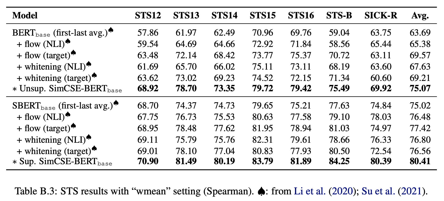 Comparison of SimCSE, BERT-flow, and BERT-whitening
However you slice it, SimCSE clearly outperforms both BERT-flow and BERT-whitening. So is this advantage of SimCSE universal? Does it hold on Chinese as well? Let's find out with some experiments.
Experimental Setup
Our Chinese experiments largely follow the setup in Which Approach Wins at Unsupervised Semantic Similarity? A Fairly Comprehensive Evaluation, including the 5 tasks tested previously, the 4 pooling methods, and all the base, small, and tiny model versions. Large models weren't tested because, under the same configuration, the large model ran out of memory (OOM).
Open-source code: https://github.com/bojone/SimCSE
After tuning, I found that the optimal hyperparameters for SimCSE on Chinese tasks don't fully match those in the original paper. The specific differences are:
1. The original paper uses batch_size=512; here we use batch_size=64 (I really can't afford such an extravagant batch size);
2. The original paper's learning rate is 5e-5; here it's 1e-5;
3. The original paper's optimal dropout ratio is 0.1; here it's 0.3;
4. The original paper's unsupervised SimCSE is trained on extra data; here we simply randomly sampled 10,000 pieces of task data for training;
5. The original paper's unsupervised training also included an MLM task; here only the SimCSE objective is used.
A further note on the last point: the original paper's unsupervised SimCSE was trained on 1 million sentences selected from Wikipedia. For our Chinese experiments, for convenience and fairness of comparison, we directly used the task data for training (using only the sentences, not the labels — still unsupervised). Except for PAWSX, none of the other 4 tasks require using all the data for training; through testing, randomly sampling 10,000 training examples and training for one epoch is sufficient to reach the optimal result (using more or fewer samples both degrade performance).
Results on Chinese
All the Chinese experimental results for SimCSE are as follows:
$$\small{\begin{array}{l|ccccc} \hline & \text{ATEC} & \text{BQ} & \text{LCQMC} & \text{PAWSX} & \text{STS-B} \\ \hline \text{BERT}\text{-P1} & 16.59 / 20.61 / \color{green}{33.14} & 29.35 / 25.76 / \color{green}{50.67} & 41.71 / 48.92 / \color{green}{69.99} & 15.15 / 17.03 / \color{red}{12.95} & 34.65 / 61.19 / \color{green}{69.04} \\ \text{BERT}\text{-P2} & 9.46 / 22.16 / \color{green}{25.18} & 16.97 / 18.97 / \color{green}{41.19} & 28.42 / 49.61 / \color{green}{56.45} & 13.93 / 16.08 / \color{red}{12.46} & 21.66 / 60.75 / \color{red}{57.63} \\ \text{BERT}\text{-P3} & 20.79 / 18.27 / \color{green}{32.89} & 33.08 / 22.58 / \color{green}{49.58} & 59.22 / 60.12 / \color{green}{71.83} & 16.68 / 18.37 / \color{red}{14.47} & 57.48 / 63.97 / \color{green}{70.08} \\ \text{BERT}\text{-P4} & 24.51 / 27.00 / \color{green}{31.96} & 38.81 / 32.29 / \color{green}{48.40} & 64.75 / 64.75 / \color{green}{71.49} & 15.12 / 17.80 / \color{red}{16.01} & 61.66 / 69.45 / \color{green}{70.03} \\ \hline \text{RoBERTa}\text{-P1} & 24.61 / 29.59 / \color{green}{32.23} & 40.54 / 28.95 / \color{green}{50.61} & 70.55 / 70.82 / \color{green}{74.22} & 16.23 / 17.99 / \color{red}{12.25} & 66.91 / 69.19 / \color{green}{71.13} \\ \text{RoBERTa}\text{-P2} & 20.61 / 28.91 / \color{red}{20.07} & 31.14 / 27.48 / \color{green}{39.92} & 65.43 / 70.62 / \color{red}{62.65} & 15.71 / 17.30 / \color{red}{12.00} & 59.50 / 70.77 / \color{red}{61.49} \\ \text{RoBERTa}\text{-P3} & 26.94 / 29.94 / \color{green}{32.66} & 40.71 / 30.95 / \color{green}{51.03} & 66.80 / 68.00 / \color{green}{73.15} & 16.08 / 19.01 / \color{red}{16.47} & 61.67 / 66.19 / \color{green}{70.14} \\ \text{RoBERTa}\text{-P4} & 27.94 / 28.33 / \color{green}{32.40} & 43.09 / 33.49 / \color{green}{49.78} & 68.43 / 67.86 / \color{green}{72.74} & 15.02 / 17.91 / \color{red}{16.39} & 64.09 / 69.74 / \color{green}{70.11} \\ \hline \text{NEZHA}\text{-P1} & 17.39 / 18.83 / \color{green}{32.14} & 29.63 / 21.94 / \color{green}{46.08} & 40.60 / 50.52 / \color{green}{60.38} & 14.90 / 18.15 / \color{red}{16.60} & 35.84 / 60.84 / \color{green}{68.50} \\ \text{NEZHA}\text{-P2} & 10.96 / 23.08 / \color{red}{15.70} & 17.38 / 28.81 / \color{green}{32.20} & 22.66 / 49.12 / \color{red}{21.07} & 13.45 / 18.05 / \color{red}{12.68} & 21.16 / 60.11 / \color{red}{43.35} \\ \text{NEZHA}\text{-P3} & 23.70 / 21.93 / \color{green}{31.47} & 35.44 / 22.44 / \color{green}{46.69} & 60.94 / 62.10 / \color{green}{69.65} & 18.35 / 21.72 / \color{red}{18.17} & 60.35 / 68.57 / \color{green}{70.68} \\ \text{NEZHA}\text{-P4} & 27.72 / 25.31 / \color{green}{30.26} & 44.18 / 31.47 / \color{green}{46.57} & 65.16 / 66.68 / \color{green}{67.21} & 13.98 / 16.66 / \color{red}{14.41} & 61.94 / 69.55 / \color{red}{68.18} \\ \hline \text{WoBERT}\text{-P1} & 23.88 / 22.45 / \color{green}{32.66} & 43.08 / 32.52 / \color{green}{49.13} & 68.56 / 67.89 / \color{green}{72.99} & 18.15 / 19.92 / \color{red}{12.36} & 64.12 / 66.53 / \color{green}{70.00} \\ \text{WoBERT}\text{-P2} & \text{-} & \text{-} & \text{-} & \text{-} & \text{-} \\ \text{WoBERT}\text{-P3} & 24.62 / 22.74 / \color{green}{34.03} & 40.64 / 28.12 / \color{green}{49.77} & 64.89 / 65.22 / \color{green}{72.44} & 16.83 / 20.56 / \color{red}{14.55} & 59.43 / 66.57 / \color{green}{70.96} \\ \text{WoBERT}\text{-P4} & 25.97 / 27.24 / \color{green}{33.67} & 42.37 / 32.34 / \color{green}{49.09} & 66.53 / 65.62 / \color{green}{71.74} & 15.54 / 18.85 / \color{red}{14.00} & 61.37 / 68.11 / \color{green}{70.00} \\ \hline \text{RoFormer}\text{-P1} & 24.29 / 26.04 / \color{green}{32.33} & 41.91 / 28.13 / \color{green}{49.13} & 64.87 / 60.92 / \color{green}{71.61} & 20.15 / 23.08 / \color{red}{15.25} & 59.91 / 66.96 / \color{green}{69.45} \\ \text{RoFormer}\text{-P2} & \text{-} & \text{-} & \text{-} & \text{-} & \text{-} \\ \text{RoFormer}\text{-P3} & 24.09 / 28.51 / \color{green}{34.23} & 39.09 / 34.92 / \color{green}{50.01} & 63.55 / 63.85 / \color{green}{72.01} & 16.53 / 18.43 / \color{red}{15.25} & 58.98 / 55.30 / \color{green}{71.44} \\ \text{RoFormer}\text{-P4} & 25.92 / 27.38 / \color{green}{34.10} & 41.75 / 32.36 / \color{green}{49.58} & 66.18 / 65.45 / \color{green}{71.84} & 15.30 / 18.36 / \color{red}{15.17} & 61.40 / 68.02 / \color{green}{71.40} \\ \hline \text{SimBERT}\text{-P1} & 38.50 / 23.64 / \color{green}{36.98} & 48.54 / 31.78 / \color{green}{51.47} & 76.23 / 75.05 / \color{red}{74.87} & 15.10 / 18.49 / \color{red}{12.66} & 74.14 / 73.37 / \color{green}{75.12} \\ \text{SimBERT}\text{-P2} & 38.93 / 27.06 / \color{green}{37.00} & 49.93 / 35.38 / \color{green}{50.33} & 75.56 / 73.45 / \color{red}{72.61} & 14.52 / 18.51 / \color{green}{19.72} & 73.18 / 73.43 / \color{green}{75.13} \\ \text{SimBERT}\text{-P3} & 36.50 / 31.32 / \color{green}{37.81} & 45.78 / 29.17 / \color{green}{51.24} & 74.42 / 73.79 / \color{green}{73.85} & 15.33 / 18.39 / \color{red}{12.48} & 67.31 / 70.70 / \color{green}{73.18} \\ \text{SimBERT}\text{-P4} & 33.53 / 29.04 / \color{green}{36.93} & 45.28 / 34.70 / \color{green}{50.09} & 73.20 / 71.22 / \color{green}{73.42} & 14.16 / 17.32 / \color{red}{16.59} & 66.98 / 70.55 / \color{green}{72.64} \\ \hline \text{SimBERT}_{\text{small}}\text{-P1} & 30.68 / 27.56 / \color{green}{31.16} & 43.41 / 30.89 / \color{green}{44.80} & 74.73 / 73.21 / \color{green}{74.32} & 15.89 / 17.96 / \color{red}{14.69} & 70.54 / 71.39 / \color{red}{69.85} \\ \text{SimBERT}_{\text{small}}\text{-P2} & 31.00 / 29.14 / \color{green}{30.76} & 43.76 / 36.86 / \color{green}{45.50} & 74.21 / 73.14 / \color{green}{74.55} & 16.17 / 18.12 / \color{red}{15.18} & 70.10 / 71.40 / \color{red}{69.18} \\ \text{SimBERT}_{\text{small}}\text{-P3} & 30.03 / 21.24 / \color{green}{30.07} & 43.72 / 31.69 / \color{green}{44.27} & 72.12 / 70.27 / \color{green}{71.21} & 16.93 / 21.68 / \color{red}{12.10} & 66.55 / 66.11 / \color{red}{64.95} \\ \text{SimBERT}_{\text{small}}\text{-P4} & 29.52 / 28.41 / \color{green}{28.56} & 43.52 / 36.56 / \color{green}{43.38} & 70.33 / 68.75 / \color{red}{68.35} & 15.39 / 21.57 / \color{red}{14.47} & 64.73 / 68.12 / \color{red}{63.23} \\ \hline \text{SimBERT}_{\text{tiny}}\text{-P1} & 30.51 / 24.67 / \color{green}{30.04} & 44.25 / 31.75 / \color{green}{43.89} & 74.27 / 72.25 / \color{green}{73.47} & 16.01 / 18.07 / \color{red}{12.51} & 70.11 / 66.39 / \color{green}{70.11} \\ \text{SimBERT}_{\text{tiny}}\text{-P2} & 30.01 / 27.66 / \color{green}{29.37} & 44.47 / 37.33 / \color{green}{44.04} & 73.98 / 72.31 / \color{green}{72.93} & 16.55 / 18.15 / \color{red}{13.73} & 70.35 / 70.88 / \color{red}{69.63} \\ \text{SimBERT}_{\text{tiny}}\text{-P3} & 28.47 / 19.68 / \color{green}{28.08} & 42.04 / 29.49 / \color{green}{41.21} & 69.16 / 66.99 / \color{green}{69.85} & 16.18 / 20.11 / \color{red}{12.21} & 64.41 / 66.72 / \color{red}{64.62} \\ \text{SimBERT}_{\text{tiny}}\text{-P4} & 27.77 / 27.67 / \color{red}{26.25} & 41.76 / 37.02 / \color{green}{41.62} & 67.55 / 65.66 / \color{green}{67.34} & 15.06 / 20.49 / \color{red}{13.87} & 62.92 / 66.77 / \color{red}{60.80} \\ \hline \end{array}}$$
Each cell contains data in the form "a/b/c," where a is the raw result with no processing applied, b is the BERT-whitening result (without dimensionality reduction), and c is the SimCSE result. If c > b, then c is shown in green; otherwise it's shown in red. In other words, the more green there is, the more SimCSE outperforms BERT-whitening. For other experimental details, see the original code as well as Which Approach Wins at Unsupervised Semantic Similarity? A Fairly Comprehensive Evaluation.
Note that, because Dropout is involved and training samples 10,000 examples randomly, the results carry some randomness — re-running the code will certainly produce fluctuations in the metrics, so readers should be aware of this.
Some Conclusions
The experimental results show that, aside from the "outlier" task PAWSX, SimCSE indeed has an overwhelming advantage over BERT-whitening, sometimes by more than 10 points on some tasks. On BQ, SimCSE even outperforms SimBERT, which was trained with supervision — and remarkably, even a model like SimBERT that has already undergone supervised training can still be further improved. All of this really demonstrates SimCSE's strength. (As for why PAWSX is an "outlier," a brief analysis was already given in Which Approach Wins at Unsupervised Semantic Similarity? A Fairly Comprehensive Evaluation.)
We can also see that, under SimCSE, the first-last-avg pooling method, which performed well under BERT-flow and BERT-whitening, no longer has any advantage. Instead, simply taking the [CLS] vector performs better. Surprisingly though, the Pooler (which adds a Dense layer on top of [CLS]) performs relatively poorly — quite puzzling.
Since BERT-whitening is just a linear transformation, I also experimented with whether SimCSE alone could reproduce the effect of this linear transformation. Specifically, I fixed the Encoder's weights and added a Dense layer with no activation function on top, then trained only this final Dense layer with the SimCSE objective. It turned out that in this setting SimCSE performs worse than BERT-whitening. This implies that for SimCSE to be effective, the Encoder itself must be fine-tuned, which also suggests that BERT-whitening may capture something that SimCSE does not. Perhaps combining the two in some way could yield even better results (still thinking this through...).
Related Work
After a quick survey, I found that the idea of "using the sample itself as its own positive pair" has appeared in several recent papers. Besides SimCSE, there's also Augmented SBERT: Data Augmentation Method for Improving Bi-Encoders for Pairwise Sentence Scoring Tasks and Semantic Re-tuning with Contrastive Tension, both of which are extremely similar in spirit. Actually, I had thought of similar ideas myself, but I never expected it would really work (so I never ran the experiments), and I certainly never guessed that the key ingredient was Dropout. Looks like there's really no substitute for running the experiments.
Summary
This post shared my Chinese-language experiments with SimCSE. The results show that on quite a few tasks, SimCSE is indeed excellent, clearly outperforming BERT-whitening.
Translated automatically with claude-sonnet-5; all equations are reproduced verbatim from the source. Copyright remains with the original author.