Rambling on about Generative Diffusion Models (16): W-distance ≤ Score Matching

生成扩散模型漫谈（十六）：W距离 ≤ 得分匹配 苏剑林 · 2023-02-14 · Machine Learning differential equation GAN generative model diffusion

The Wasserstein distance (henceforth "W-distance") is a distance function that measures the discrepancy between two probability distributions based on the idea of optimal transport. I've introduced it before in posts such as From the Wasserstein Distance and Duality Theory to WGAN. For many readers, the first time they heard of the W-distance was probably through WGAN, which appeared in 2017 and opened up a new line of research on understanding GANs from the perspective of optimal transport, while also raising the profile of optimal transport theory within machine learning. For a long time, GANs were the "main force" in the field of generative models, and it was only in the past couple of years, with the meteoric rise of diffusion models, that GANs' prominence has somewhat faded — though they remain a powerful class of generative model in their own right.

On the surface, diffusion models and GANs look quite different, so research on the two has largely proceeded independently. However, a paper from late last year, Score-based Generative Modeling Secretly Minimizes the Wasserstein Distance, broke down this divide: it proves that the score matching loss of diffusion models can be written as an upper bound on the W-distance. This means that, in some sense, minimizing the loss function of a diffusion model is — just like with WGAN — actually minimizing the W-distance between two distributions.more

Analyzing the Conclusion

Specifically, the original paper's result concerns the SDE-based diffusion models introduced in Rambling on about Generative Diffusion Models (5): The General SDE Framework. Its core conclusion is the inequality (where $I_t$ is a non-negative function of $t$, whose precise meaning we'll explain in detail later)

\begin{equation}\mathcal{W}_2[p_0,q_0]\leq \int_0^T g_t^2 I_t \left(\mathbb{E}_{\boldsymbol{x}_t\sim p_t(\boldsymbol{x}_t)}\left[\left\Vert\nabla_{\boldsymbol{x}_t}\log p(\boldsymbol{x}_t) - \boldsymbol{s}_{\boldsymbol{\theta}}(\boldsymbol{x}_t,t)\right\Vert^2\right]\right)^{1/2}dt + I_T \mathcal{W}_2[p_T,q_T]\label{eq:w-neq}\end{equation}

So how should we understand this inequality? First, a diffusion model can be understood as an SDE process moving from $t=T$ to $t=0$, and the rightmost term $p_T,q_T$ is the distribution of random samples at time $T$; $p_T$ is usually the standard normal distribution, and in practice we typically have $q_T = p_T$, so $\mathcal{W}_2[p_T,q_T]=0$. The original paper writes it out explicitly only to give the most general result at the theoretical level.

Next, the left-hand side $p_0$ is the distribution, at time $t=0$, of values obtained by starting from random points sampled at $p_T$ and solving the reverse SDE

\begin{equation}d\boldsymbol{x}_t = \left[\boldsymbol{f}_t(\boldsymbol{x}_t) - g_t^2\nabla_{\boldsymbol{x}_t}\log p_t(\boldsymbol{x}_t) \right] dt + g_t d\boldsymbol{w}\label{eq:reverse-sde}\end{equation}

This is in fact the data distribution we want to generate. Meanwhile, $q_0$ is the distribution, at time $t=0$, of values obtained by starting from random points sampled at $q_T$ and solving the SDE

\begin{equation}d\boldsymbol{x}_t = \left[\boldsymbol{f}_t(\boldsymbol{x}_t) - g_t^2\boldsymbol{s}_{\boldsymbol{\theta}}(\boldsymbol{x}_t,t) \right] dt + g_t d\boldsymbol{w}\end{equation}

where $\boldsymbol{s}_{\boldsymbol{\theta}}(\boldsymbol{x}_t,t)$ is the neural network approximation of $\nabla_{\boldsymbol{x}_t}\log p_t(\boldsymbol{x}_t)$, so $q_0$ is precisely the data distribution generated by the diffusion model. Therefore, $\mathcal{W}_2[p_0,q_0]$ is by definition the W-distance between the data distribution and the generated distribution.

Finally, the remaining integral term has as its key component

\begin{equation}\mathbb{E}_{\boldsymbol{x}_t\sim p_t(\boldsymbol{x}_t)}\left[\left\Vert\nabla_{\boldsymbol{x}_t}\log p(\boldsymbol{x}_t) - \boldsymbol{s}_{\boldsymbol{\theta}}(\boldsymbol{x}_t,t)\right\Vert^2\right]\label{eq:sm}\end{equation}

which is exactly the "score matching" loss of the diffusion model. So when we train a diffusion model using the score matching loss, we are, indirectly, also minimizing the W-distance between the data distribution and the generated distribution. The difference from WGAN is that WGAN optimizes the W-distance $\mathcal{W}_1[p_0,q_0]$, whereas here it's $\mathcal{W}_2[p_0,q_0]$.

Note:
To be precise, equation $\eqref{eq:sm}$ is not yet the actual loss function of a diffusion model — the actual loss function is the "conditional score matching" loss, whose relationship to score matching is:
\begin{equation}\begin{aligned} > &\,\mathbb{E}_{\boldsymbol{x}_t\sim p_t(\boldsymbol{x}_t)}\left[\left\Vert\nabla_{\boldsymbol{x}_t}\log p_t(\boldsymbol{x}_t) - \boldsymbol{s}_{\boldsymbol{\theta}}(\boldsymbol{x}_t,t)\right\Vert^2\right] \\ > =&\,\mathbb{E}_{\boldsymbol{x}_t\sim p_t(\boldsymbol{x}_t)}\left[\left\Vert\mathbb{E}_{\boldsymbol{x}_0\sim p_t(\boldsymbol{x}_0|\boldsymbol{x}_t)}\left[\nabla_{\boldsymbol{x}_t}\log p_t(\boldsymbol{x}_t|\boldsymbol{x}_0)\right] - \boldsymbol{s}_{\boldsymbol{\theta}}(\boldsymbol{x}_t,t)\right\Vert^2\right] \\ > \leq &\,\mathbb{E}_{\boldsymbol{x}_t\sim p_t(\boldsymbol{x}_t)}\mathbb{E}_{\boldsymbol{x}_0\sim p_t(\boldsymbol{x}_0|\boldsymbol{x}_t)}\left[\left\Vert\nabla_{\boldsymbol{x}_t}\log p_t(\boldsymbol{x}_t|\boldsymbol{x}_0) - \boldsymbol{s}_{\boldsymbol{\theta}}(\boldsymbol{x}_t,t)\right\Vert^2\right] \\ > = &\,\mathbb{E}_{\boldsymbol{x}_0\sim p_0(\boldsymbol{x}_0),\boldsymbol{x}_t\sim p_t(\boldsymbol{x}_t|\boldsymbol{x}_0)}\left[\left\Vert\nabla_{\boldsymbol{x}_t}\log p_t(\boldsymbol{x}_t|\boldsymbol{x}_0) - \boldsymbol{s}_{\boldsymbol{\theta}}(\boldsymbol{x}_t,t)\right\Vert^2\right] \\ > \end{aligned}\end{equation}
The final result is the diffusion model's loss function, "conditional score matching." The first equality follows from the identity $\nabla_{\boldsymbol{x}_t}\log p_t(\boldsymbol{x}_t)=\mathbb{E}_{\boldsymbol{x}_0\sim p_t(\boldsymbol{x}_0|\boldsymbol{x}_t)}\left[\nabla_{\boldsymbol{x}_t}\log p_t(\boldsymbol{x}_t|\boldsymbol{x}_0)\right]$, the second inequality follows from a generalization of the quadratic-mean inequality (or Jensen's inequality), and the third equality is Bayes' rule. In other words, conditional score matching is an upper bound on score matching, and is therefore also an upper bound on the W-distance.

From equation $\eqref{eq:w-neq}$ we can also get a simple intuition for why the diffusion model's objective function drops the coefficient in front of the squared norm: since the W-distance is a well-behaved measure of the discrepancy between probability distributions, and the right-hand side of $\eqref{eq:w-neq}$ contains $g_t^2 I_t$, which is a monotonically increasing function of $t$, this means we should appropriately upweight the score matching loss when $t$ is small. In Rambling on about Generative Diffusion Models (5): The General SDE Framework we derived that the final form of score matching is:

\begin{equation}\frac{1}{\bar{\beta}_t^2}\mathbb{E}_{\boldsymbol{x}_0\sim \tilde{p}(\boldsymbol{x}_0),\boldsymbol{\varepsilon}\sim\mathcal{N}(\boldsymbol{0},\boldsymbol{I})}\left[\left\Vert \boldsymbol{\epsilon}_{\boldsymbol{\theta}}(\bar{\alpha}_t\boldsymbol{x}_0 + \bar{\beta}_t\boldsymbol{\varepsilon}, t) - \boldsymbol{\varepsilon}\right\Vert^2\right]\end{equation}

Dropping the coefficient $\frac{1}{\bar{\beta}_t^2}$ is equivalent to multiplying by $\bar{\beta}_t^2$, and $\bar{\beta}_t^2$ is likewise a monotonically increasing function of $t$. In other words, we can simply think of dropping this coefficient as a way of making the training objective closer to the W-distance between the two distributions.

Preliminaries

Although the original paper provides a proof of inequality $\eqref{eq:w-neq}$, it draws on a considerable amount of optimal transport theory — continuity equations, gradient flows, and so on. In particular, it cites without proof a theorem that appears buried in Chapter 8 of a monograph on gradient flows, or Chapter 5 of another monograph on optimal transport — both of which were quite hard going for me. After some time spent working through it, I finally completed, last week, my own (partial) proof of inequality $\eqref{eq:w-neq}$, using nothing more than the definition of the W-distance, basic differential equations, and the Cauchy–Schwarz inequality. This should be noticeably easier to follow than the original paper's proof. After a few days of revision, here is the proof.

Before starting the proof, let's do some preparatory work and review a few basic concepts and results we'll need. First, the W-distance, defined as

\begin{equation}\mathcal{W}_{\rho}[p,q]=\left(\inf_{\gamma\in \Pi[p,q]} \iint \gamma(\boldsymbol{x},\boldsymbol{y}) \Vert\boldsymbol{x} - \boldsymbol{y}\Vert^{\rho} d\boldsymbol{x}d\boldsymbol{y}\right)^{1/\rho}\end{equation}

where $\Pi[p,q]$ refers to the set of all joint probability density functions with $p,q$ as marginals, describing a specific transport plan. This post only considers $\rho=2$, since only this case is convenient for what follows. Note that the definition of the W-distance involves an infimum $\inf$, which means that for any $\gamma\in \Pi[p,q]$ we can construct, we have

\begin{equation}\mathcal{W}_2[p,q]\leq\left(\iint \gamma(\boldsymbol{x},\boldsymbol{y}) \Vert\boldsymbol{x} - \boldsymbol{y}\Vert^{2} d\boldsymbol{x}d\boldsymbol{y}\right)^{1/2}\label{eq:core-neq}\end{equation}

This is the core idea of the proof presented here. The bounding steps in the proof mainly rely on the Cauchy–Schwarz inequality:

\begin{equation}\begin{aligned} &\text{vector version:}\quad\boldsymbol{x}\cdot\boldsymbol{y}\leq \Vert \boldsymbol{x}\Vert \Vert\boldsymbol{y}\Vert\\ &\text{expected version:}\quad\mathbb{E}_{\boldsymbol{x}}\left[f(\boldsymbol{x})g(\boldsymbol{x})\right]\leq \left(\mathbb{E}_{\boldsymbol{x}}\left[f^2(\boldsymbol{x})\right]\right)^{1/2}\left(\mathbb{E}_{\boldsymbol{x}}\left[g^2(\boldsymbol{x})\right]\right)^{1/2} \end{aligned}\end{equation}

In the course of the proof we will assume that the function $\boldsymbol{g}_t(\boldsymbol{x})$ satisfies a "one-sided Lipschitz constraint," defined as

\begin{equation}(\boldsymbol{g}_t(\boldsymbol{x}) - \boldsymbol{g}_t(\boldsymbol{y}))\cdot(\boldsymbol{x} - \boldsymbol{y}) \leq L_t \Vert \boldsymbol{x} - \boldsymbol{y}\Vert^2\label{eq:assum}\end{equation}

It can be shown that this is weaker than the usual Lipschitz constraint (see Lipschitz Constraints in Deep Learning: Generalization and Generative Models), i.e., if a function $\boldsymbol{g}_t(\boldsymbol{x})$ satisfies the Lipschitz constraint, it necessarily satisfies the one-sided Lipschitz constraint.

A First Attempt

Inequality $\eqref{eq:w-neq}$ is too general — trying to analyze the general result straight away isn't conducive to clear thinking. So let's first simplify the problem and see whether we can prove a somewhat weaker result. How do we simplify it? First, inequality $\eqref{eq:w-neq}$ considers the discrepancy between initial distributions (recall that in a diffusion model, the process runs from $t=T$ to $t=0$, so $t=T$ is the initial time and $t=0$ is the terminal time); here we'll first consider the case of identical initial distributions. Also, the original reverse equation $\eqref{eq:reverse-sde}$ is an SDE; here we'll first consider the deterministic ODE case.

Specifically, we consider sampling $\boldsymbol{z}$ from the same distribution $q(\boldsymbol{z})$ as the initial value at time $T$, and then evolving it forward along two different ODEs:

\begin{equation}\frac{d\boldsymbol{x}_t}{dt} = \boldsymbol{f}_t(\boldsymbol{x}_t),\quad \frac{d\boldsymbol{y}_t}{dt} = \boldsymbol{g}_t(\boldsymbol{y}_t)\end{equation}

Let the distribution of $\boldsymbol{x}_t$ at time $t$ be $p_t$, and the distribution of $\boldsymbol{y}_t$ be $q_t$. We'll try to estimate an upper bound for $\mathcal{W}_2[p_0,q_0]$.

We know that $\boldsymbol{x}_t,\boldsymbol{y}_t$ are both obtained by evolving from the same initial value $\boldsymbol{z}$ via their respective ODEs, so they are actually both deterministic functions of $\boldsymbol{z}$ — more precisely they should be written $\boldsymbol{x}_t(\boldsymbol{z}),\boldsymbol{y}_t(\boldsymbol{z})$, but for simplicity we omit $\boldsymbol{z}$. This means that, for each fixed $\boldsymbol{x}$, $\boldsymbol{x}_t\leftrightarrow \boldsymbol{y}_t$ constitutes a correspondence (a transport plan) between the samples of $p_t,q_t$, as illustrated below (this diagram wasn't easy to draw, so I just sketched it by hand):

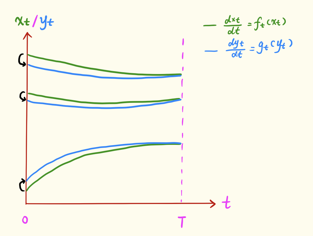Illustration of an approximate optimal transport plan

So from equation $\eqref{eq:core-neq}$, we can write

\begin{equation}\mathcal{W}_2^2[p_t,q_t]\leq \mathbb{E}_{\boldsymbol{z}}\left[\Vert\boldsymbol{x}_t - \boldsymbol{y}_t\Vert^{2} \right]\triangleq \tilde{\mathcal{W}}_2^2[p_t,q_t]\label{eq:core-neq-2}\end{equation}

Next we bound $\tilde{\mathcal{W}}_2^2[p_t,q_t]$. To connect it with $\boldsymbol{f}_t(\boldsymbol{x}_t),\boldsymbol{g}_t(\boldsymbol{y}_t)$, we differentiate it:

\begin{equation}\begin{aligned} \pm\frac{d\left(\tilde{\mathcal{W}}_2^2[p_t,q_t]\right)}{dt}=&\, \pm2\mathbb{E}_{\boldsymbol{z}}\left[(\boldsymbol{x}_t - \boldsymbol{y}_t)\cdot \left(\frac{d\boldsymbol{x}_t}{dt} - \frac{d\boldsymbol{y}_t}{dt}\right)\right] \\[5pt] =&\, \pm 2\mathbb{E}_{\boldsymbol{z}}\left[(\boldsymbol{x}_t - \boldsymbol{y}_t)\cdot (\boldsymbol{f}_t(\boldsymbol{x}_t) - \boldsymbol{g}_t(\boldsymbol{y}_t))\right] \\[5pt] =&\, \pm 2\mathbb{E}_{\boldsymbol{z}}\left[(\boldsymbol{x}_t - \boldsymbol{y}_t)\cdot (\boldsymbol{f}_t(\boldsymbol{x}_t) - \boldsymbol{g}_t(\boldsymbol{x}_t))\right] \pm 2\mathbb{E}_{\boldsymbol{z}}\left[(\boldsymbol{x}_t - \boldsymbol{y}_t)\cdot (\boldsymbol{g}_t(\boldsymbol{x}_t) - \boldsymbol{g}_t(\boldsymbol{y}_t))\right] \\[5pt] \leq&\, 2\mathbb{E}_{\boldsymbol{z}}\left[\Vert\boldsymbol{x}_t - \boldsymbol{y}_t\Vert \Vert\boldsymbol{f}_t(\boldsymbol{x}_t) - \boldsymbol{g}_t(\boldsymbol{x}_t)\Vert\right] + 2\mathbb{E}_{\boldsymbol{z}}\left[L_t\Vert\boldsymbol{x}_t - \boldsymbol{y}_t\Vert^2\right] \\[5pt] \leq&\, 2\left(\mathbb{E}_{\boldsymbol{z}}\left[\Vert\boldsymbol{x}_t - \boldsymbol{y}_t\Vert^2\right]\right)^{1/2} \left(\mathbb{E}_{\boldsymbol{z}}\left[\Vert\boldsymbol{f}_t(\boldsymbol{x}_t) - \boldsymbol{g}_t(\boldsymbol{x}_t)\Vert^2\right]\right)^{1/2} + 2L_t\mathbb{E}_{\boldsymbol{z}}\left[\Vert\boldsymbol{x}_t - \boldsymbol{y}_t\Vert^2\right] \\[5pt] =&\, 2 \tilde{\mathcal{W}}_2[p_t,q_t] \left(\mathbb{E}_{\boldsymbol{z}}\left[\Vert\boldsymbol{f}_t(\boldsymbol{x}_t) - \boldsymbol{g}_t(\boldsymbol{x}_t)\Vert^2\right]\right)^{1/2} + 2L_t\tilde{\mathcal{W}}_2^2[p_t,q_t] \\[5pt] \end{aligned}\label{eq:der-neq-0}\end{equation}

where the first inequality uses the vector version of the Cauchy–Schwarz inequality together with the one-sided Lipschitz constraint assumption $\eqref{eq:assum}$, and the second inequality uses the expectation version of the Cauchy–Schwarz inequality. Here $\pm$ means that the resulting inequality holds regardless of whether we take $+$ or $-$; the derivation below only makes use of the $-$ side. Combining with $\left(w^2\right)'=2ww'$, we obtain

\begin{equation}-\frac{d\tilde{\mathcal{W}}_2[p_t,q_t]}{dt} \leq \left(\mathbb{E}_{\boldsymbol{z}}\left[\Vert\boldsymbol{f}_t(\boldsymbol{x}_t) - \boldsymbol{g}_t(\boldsymbol{x}_t)\Vert^2\right]\right)^{1/2} + L_t\tilde{\mathcal{W}}_2[p_t,q_t] \label{eq:der-neq-1}\end{equation}

Using the method of variation of parameters, let $\tilde{\mathcal{W}}_2[p_t,q_t]=C_t \exp\left(\int_t^T L_s ds\right)$; substituting into the equation above gives

\begin{equation}-\frac{dC_t}{dt} \leq \exp\left(-\int_t^T L_s ds\right)\left(\mathbb{E}_{\boldsymbol{z}}\left[\Vert\boldsymbol{f}_t(\boldsymbol{x}_t) - \boldsymbol{g}_t(\boldsymbol{x}_t)\Vert^2\right]\right)^{1/2}\label{eq:der-neq-2}\end{equation}

Integrating both sides over $[0,T]$, and using $C_T=0$ (the two distributions coincide at the initial time, so the distance is 0), we get

\begin{equation}C_0 \leq \int_0^T \exp\left(-\int_t^T L_s ds\right)\left(\mathbb{E}_{\boldsymbol{z}}\left[\Vert\boldsymbol{f}_t(\boldsymbol{x}_t) - \boldsymbol{g}_t(\boldsymbol{x}_t)\Vert^2\right]\right)^{1/2} dt\end{equation}

which gives us

\begin{equation}\tilde{\mathcal{W}}_2[p_0,q_0] \leq C_0 \exp\left(\int_0^T L_s ds\right) =\int_0^T I_t\left(\mathbb{E}_{\boldsymbol{z}}\left[\Vert\boldsymbol{f}_t(\boldsymbol{x}_t) - \boldsymbol{g}_t(\boldsymbol{x}_t)\Vert^2\right]\right)^{1/2} dt\end{equation}

where $I_t = \exp\left(\int_0^t L_s ds\right)$. By equation $\eqref{eq:core-neq-2}$, this is also an upper bound on $\mathcal{W}_2[p_0,q_0]$. Finally, since the expectation expression is a function of $\boldsymbol{x}_t$ only, and $\boldsymbol{x}_t$ is itself a deterministic function of $\boldsymbol{z}$, the expectation with respect to $\boldsymbol{z}$ is equivalent to taking the expectation directly with respect to $\boldsymbol{x}_t$, so:

\begin{equation}\mathcal{W}_2[p_0,q_0] \leq\int_0^T I_t\left(\mathbb{E}_{\boldsymbol{x}_t\sim p_t(\boldsymbol{x}_t)}\left[\Vert\boldsymbol{f}_t(\boldsymbol{x}_t) - \boldsymbol{g}_t(\boldsymbol{x}_t)\Vert^2\right]\right)^{1/2} dt\label{eq:w-neq-0}\end{equation}

Pressing On

In fact, the simplified inequality $\eqref{eq:w-neq-0}$ is already essentially no different from the more general $\eqref{eq:w-neq}$: its derivation already contains the general strategy needed to obtain the full result. Let's now complete the remaining derivation.

First, we extend equation $\eqref{eq:w-neq-0}$ to the setting of different initial distributions. Suppose we have two initial distributions $p_T(\boldsymbol{z}_1),q_T(\boldsymbol{z}_2)$: from $p_T(\boldsymbol{z}_1)$ we sample an initial value and evolve it via $\boldsymbol{x}_t$, and from $q_T(\boldsymbol{z}_2)$ we sample an initial value and evolve it via $\boldsymbol{y}_t$. So now $\boldsymbol{x}_t,\boldsymbol{y}_t$ are functions of $\boldsymbol{z}_1,\boldsymbol{z}_2$ respectively, rather than functions of the same $\boldsymbol{z}$ as before, so we can't directly construct a transport plan. We therefore need a correspondence (transport plan) between $\boldsymbol{z}_1,\boldsymbol{z}_2$, which we choose to be an optimal transport plan $\gamma^*(\boldsymbol{z}_1,\boldsymbol{z}_2)$ between $p_T(\boldsymbol{z}_1),q_T(\boldsymbol{z}_2)$. This lets us write a result analogous to equation $\eqref{eq:core-neq-2}$:

\begin{equation}\mathcal{W}_2^2[p_t,q_t]\leq \mathbb{E}_{\boldsymbol{z}_1,\boldsymbol{z}_2\sim \gamma^*(\boldsymbol{z}_1,\boldsymbol{z}_2)}\left[\Vert\boldsymbol{x}_t - \boldsymbol{y}_t\Vert^{2} \right]\triangleq \tilde{\mathcal{W}}_2^2[p_t,q_t]\label{eq:core-neq-3}\end{equation}

By consistency of the definitions, the bounding step $\eqref{eq:der-neq-0}$ still holds, except that the expectation $\mathbb{E}_{\boldsymbol{z}}$ is replaced by $\mathbb{E}_{\boldsymbol{z}_1,\boldsymbol{z}_2}$, so inequalities $\eqref{eq:der-neq-1}$ and $\eqref{eq:der-neq-2}$ still hold as well. The difference is that when integrating both sides of $\eqref{eq:der-neq-2}$ over $[0,T]$, we no longer have $C_T = 0$, but rather, by definition, $C_T=\tilde{\mathcal{W}}_2[p_T,q_T]=\mathcal{W}_2[p_T,q_T]$. So, the final result is

\begin{equation}\mathcal{W}_2[p_0,q_0] \leq\int_0^T I_t\left(\mathbb{E}_{\boldsymbol{x}_t\sim p_t(\boldsymbol{x}_t)}\left[\Vert\boldsymbol{f}_t(\boldsymbol{x}_t) - \boldsymbol{g}_t(\boldsymbol{x}_t)\Vert^2\right]\right)^{1/2} dt + I_T \mathcal{W}_2[p_T,q_T]\label{eq:w-neq-1}\end{equation}

Finally, let's return to diffusion models. In Rambling on about Generative Diffusion Models (6): The General ODE Framework, we've already derived that a single forward diffusion process actually corresponds to a whole family of reverse processes:

\begin{equation}d\boldsymbol{x} = \left(\boldsymbol{f}_t(\boldsymbol{x}) - \frac{1}{2}(g_t^2 + \sigma_t^2)\nabla_{\boldsymbol{x}}\log p_t(\boldsymbol{x})\right) dt + \sigma_t d\boldsymbol{w}\label{eq:sde-reverse-2}\end{equation}

where $\sigma_t$ is a freely chosen standard-deviation function; when $\sigma_t=g_t$, this reduces to equation $\eqref{eq:reverse-sde}$. Since our analysis above concerned the ODE case, let's first consider the case $\sigma_t=0$, where the result $\eqref{eq:w-neq-1}$ still applies, except with $\boldsymbol{f}_t(\boldsymbol{x}_t)$ replaced by $\boldsymbol{f}_t(\boldsymbol{x}_t) - \frac{1}{2}g_t^2\nabla_{\boldsymbol{x}_t}\log p_t(\boldsymbol{x}_t)$ and $\boldsymbol{g}_t(\boldsymbol{x}_t)$ replaced by $\boldsymbol{f}_t(\boldsymbol{x}_t) - \frac{1}{2}g_t^2\boldsymbol{s}_{\boldsymbol{\theta}}(\boldsymbol{x}_t,t)$. Substituting into equation $\eqref{eq:w-neq-1}$ then gives us the conclusion $\eqref{eq:w-neq}$ stated at the beginning of the post. Of course, we shouldn't forget the one-sided Lipschitz constraint assumption $\eqref{eq:assum}$ we made on $\boldsymbol{g}_t(\boldsymbol{x}_t)$ in the derivation — this can now be assumed separately for $\boldsymbol{f}_t(\boldsymbol{x}_t)$ and $\boldsymbol{s}_{\boldsymbol{\theta}}(\boldsymbol{x}_t,t)$, though we won't spell out these details here.

A Difficult Conclusion

Following the plan, we should now push on and finish the proof for $\sigma_t\neq 0$. Unfortunately, the approach in this post cannot fully prove the SDE case; below I'll present my analysis. In fact, for most readers, understanding the ODE example in the previous section should already be enough to grasp the essence of $\eqref{eq:w-neq-1}$ — the full details aren't all that important.

For simplicity, let's take $\eqref{eq:reverse-sde}$ as an example; the more general $\eqref{eq:sde-reverse-2}$ can be analyzed similarly. What we need to estimate is the discrepancy between the distributions of the trajectories evolved by the following two SDEs:

\begin{equation}\left\{\begin{aligned} d\boldsymbol{x}_t =&\, \left[\boldsymbol{f}_t(\boldsymbol{x}_t) - g_t^2\nabla_{\boldsymbol{x}_t}\log p_t(\boldsymbol{x}_t) \right] dt + g_t d\boldsymbol{w}\\[5pt] d\boldsymbol{y}_t =&\, \left[\boldsymbol{f}_t(\boldsymbol{y}_t) - g_t^2\boldsymbol{s}_{\boldsymbol{\theta}}(\boldsymbol{y}_t,t) \right] dt + g_t d\boldsymbol{w} \end{aligned}\right.\end{equation}

That is, we want to know how much replacing the exact $\nabla_{\boldsymbol{x}_t}\log p_t(\boldsymbol{x}_t)$ with the approximate $\boldsymbol{s}_{\boldsymbol{\theta}}(\boldsymbol{y}_t,t)$ affects the final distribution. My approach is again to convert this into an ODE and reuse the earlier proof. First, from equation $\eqref{eq:sde-reverse-2}$, we know that the ODE corresponding to the first SDE is:

\begin{equation} d\boldsymbol{x}_t = \left[\boldsymbol{f}_t(\boldsymbol{x}_t) - g_t^2\nabla_{\boldsymbol{x}_t}\log p_t(\boldsymbol{x}_t) \right] dt + g_t d\boldsymbol{w}\\ \Downarrow \\ d\boldsymbol{x}_t = \left[\boldsymbol{f}_t(\boldsymbol{x}_t) - \frac{1}{2}g_t^2\nabla_{\boldsymbol{x}_t}\log p_t(\boldsymbol{x}_t) \right] dt \end{equation}

As for the ODE corresponding to the second SDE, deriving it requires a bit of a trick: we first need to rewrite it in the form $-g_t^2\nabla_{\boldsymbol{y}_t}\log q_t(\boldsymbol{y}_t)$, and then apply equation $\eqref{eq:sde-reverse-2}$:

\begin{equation} d\boldsymbol{y}_t = \left[\boldsymbol{f}_t(\boldsymbol{y}_t) - g_t^2\boldsymbol{s}_{\boldsymbol{\theta}}(\boldsymbol{y}_t,t) \right] dt + g_t d\boldsymbol{w} \\ \Downarrow \\ d\boldsymbol{y}_t = \Big[\underbrace{\boldsymbol{f}_t(\boldsymbol{y}_t) - g_t^2\boldsymbol{s}_{\boldsymbol{\theta}}(\boldsymbol{y}_t,t) + g_t^2\nabla_{\boldsymbol{y}_t}\log q_t(\boldsymbol{y}_t)}_{\text{treat as whole}} - g_t^2\nabla_{\boldsymbol{y}_t}\log q_t(\boldsymbol{y}_t) \Big] dt + g_t d\boldsymbol{w} \\ \Downarrow \\ d\boldsymbol{y}_t = \left[\boldsymbol{f}_t(\boldsymbol{y}_t) - g_t^2\boldsymbol{s}_{\boldsymbol{\theta}}(\boldsymbol{y}_t,t) + g_t^2\nabla_{\boldsymbol{y}_t}\log q_t(\boldsymbol{y}_t) - \frac{1}{2}g_t^2\nabla_{\boldsymbol{y}_t}\log q_t(\boldsymbol{y}_t) \right] dt \\ \Downarrow \\ d\boldsymbol{y}_t = \left[\boldsymbol{f}_t(\boldsymbol{y}_t) - g_t^2\boldsymbol{s}_{\boldsymbol{\theta}}(\boldsymbol{y}_t,t) + \frac{1}{2}g_t^2\nabla_{\boldsymbol{y}_t}\log q_t(\boldsymbol{y}_t)\right] dt \end{equation}

Repeating the bounding process $\eqref{eq:der-neq-0}$ for these two ODEs (taking the negative sign for $\pm$), the main difference is an extra term:

\begin{equation}-\frac{1}{2}g_t^2\mathbb{E}_{\boldsymbol{z}}\left[(\boldsymbol{x}_t - \boldsymbol{y}_t)\cdot (\nabla_{\boldsymbol{x}_t}\log p_t(\boldsymbol{x}_t)-\nabla_{\boldsymbol{y}_t}\log q_t(\boldsymbol{y}_t))\right]\end{equation}

If this term is less than or equal to 0, then the bounding step $\eqref{eq:der-neq-0}$ still holds, and all the subsequent results follow as well, with the final conclusion taking the same form as equation $\eqref{eq:w-neq-1}$.

So the remaining question is whether we can prove

\begin{equation}\mathbb{E}_{\boldsymbol{z}}\left[(\boldsymbol{x}_t - \boldsymbol{y}_t)\cdot (\nabla_{\boldsymbol{x}_t}\log p_t(\boldsymbol{x}_t)-\nabla_{\boldsymbol{y}_t}\log q_t(\boldsymbol{y}_t))\right]\geq 0\end{equation}

Unfortunately, one can construct counterexamples showing that this does not hold in general. A similar term appears in the original paper's proof, except the expectation is taken not with respect to $\boldsymbol{z}$, but with respect to the optimal transport distribution between $\boldsymbol{x}_t,\boldsymbol{y}_t$. Under this assumption, the original paper simply invokes the conclusions of two references as lemmas, completing the proof in just a few lines. I have to say the authors of the original paper are clearly very much at home with optimal transport — pulling in results from various references with ease — which makes life hard for a novice reader like me, who wants to understand things thoroughly but finds it difficult to get a real foothold. I'll have to stop here.

It's worth stressing that we cannot impose a one-sided Lipschitz constraint on either $\nabla_{\boldsymbol{x}_t}\log p_t(\boldsymbol{x}_t)$ or $\nabla_{\boldsymbol{y}_t}\log q_t(\boldsymbol{y}_t)$, since it's easy to find distributions whose log-gradient fails to satisfy the one-sided Lipschitz constraint. So, to prove this inequality, one would have to follow the original paper's approach and work from the properties of the distributions themselves, without imposing extra assumptions.

Summary

This post introduced a new theoretical result showing that the score matching loss of diffusion models can be written as an upper bound on the W-distance, and presented a partial proof of my own. This result implies that, in some sense, diffusion models and WGANs share the same optimization objective — diffusion models are secretly optimizing the W-distance too!