ChildTuning: Trying to Add Dropout to Gradients?

ChildTuning：试试把Dropout加到梯度上去？ 苏剑林 · 2021-11-22 · Machine Learning model optimization gradient

Dropout is a classic idea for preventing overfitting, one that most readers have probably already encountered. Interestingly, Dropout has recently been experiencing something of a resurgence, with several interesting new twists appearing — for example the recently much-discussed SimCSE and R-Drop. In particular, in the post Dropout Twice Again! This Time It Achieves SOTA on Supervised Tasks, we saw that this simple R-Drop approach can even rival adversarial training, which is honestly quite surprising.

Generally speaking, Dropout is applied either to the output of each layer, or to the model parameters — these are the two classic use cases. Recently, however, I learned a novel usage from the paper Raise a Child in Large Language Model: Towards Effective and Generalizable Fine-tuning: applying it to the gradients.

Dropout on the gradients? I suspect most readers have never heard of this. So how well does it actually work? Let's take a close look.more

Overview of the Method

In brief, this paper proposes an approach called "ChildTuning" to improve the fine-tuning performance of pretrained models. Here "Child" refers to "Children Network," meaning that a subnetwork is selected from the pretrained model for optimization, which mitigates the overfitting risk that comes with optimizing the entire model. The way the subnetwork is chosen splits into two variants: ChildTuning-D and ChildTuning-F.

ChildTuning-D

ChildTuning-D (Task-Dependent) is a task-dependent selection method, which requires the downstream task's training data to participate in the computation. Specifically, suppose the training data is $(x_1,y_1),(x_2,y_2),\cdots,(x_n,y_n)$ and the model is $p(y|x;\theta)$, where $\theta$ denotes all the model's parameters and $\theta_i$ is the $i$-th parameter among them. Then we compute the following form of Fisher information as the importance measure for that parameter:

\begin{equation}F_i = \frac{1}{n}\sum_{j=1}^n \left(\frac{\partial \log p(y_j|x_j;\theta)}{\partial\theta_i}\right)^2\end{equation}

Once we have this importance metric, we can rank all the parameters, and then pick out the top-$p$ most important ones (say the top 20%, i.e. $p=0.2$), and only optimize these parameters during model updates. Since fewer parameters are being optimized, the risk of overfitting is reduced. In practice, ChildTuning-D fixes the set of parameters to be optimized before fine-tuning even starts, and this selection stays fixed thereafter.

Note that the parameter selection here operates at the level of individual components — that is, within a single parameter matrix, only part of it may be selected. So we can't simply say that certain whole parameter matrices are excluded from optimization; instead, we need to construct a corresponding 0/1 matrix $M$ to mask out the corresponding gradients, i.e. $g\leftarrow g\otimes M / p$, where dividing by $p$ keeps the overall update magnitude unchanged. In this way, the gradients of unselected parameters stay at zero forever, so they never get updated. As a result, although in theory fewer parameters are being updated, this doesn't actually save any computation, which is why the authors position it purely as a way to improve fine-tuning performance rather than as an efficiency trick.

ChildTuning-F

ChildTuning-F (Task-Free) is a task-independent selection method; in fact, it can be more vividly described as "gradient Dropout." For ChildTuning-D, we build a fixed 0/1 matrix $M$ based on the task data, and then modify the gradient to $g\otimes M / p$. Since ChildTuning-F is meant to be task-independent, at every update step it instead randomly constructs a 0/1 matrix $M$, where the proportion of 1s is $p$, and then modifies the gradient to $g\otimes M / p$. As you can see, this is essentially applying Dropout to the gradient.

Note that a parameter's current gradient being zero does not mean its current update is zero, because we usually use optimizers with momentum, such as SGDM and Adam. For such optimizers, the update is proportional to the momentum, and the momentum is a running average of past gradients, i.e. $m_t = \beta m_{t-1} + (1-\beta)g_t$. So even if the current gradient is zero, as long as the parameter's historical gradients are nonzero, the momentum is still very likely to be nonzero, and thus the update will also be nonzero.

This raises a question for me: according to the design intent of ChildTuning, it seems the goal should be to select a subnetwork for updating at each step — in other words, to update only a fraction $p$ of the parameters at each step. But based on the analysis above, applying Dropout to the gradient doesn't actually achieve this goal. To truly achieve it, we should be applying Dropout to the actual update $\Delta\theta$ at each step. Yet after repeatedly reading the original paper, and even checking against the authors' open-sourced code, I've confirmed that the paper really does mean Dropout applied to the gradient.

Experimental Results

Judging from the experimental results reported in the original paper, ChildTuning's track record is quite impressive — improvements are seen almost everywhere, with the largest gain reaching as much as 8%!

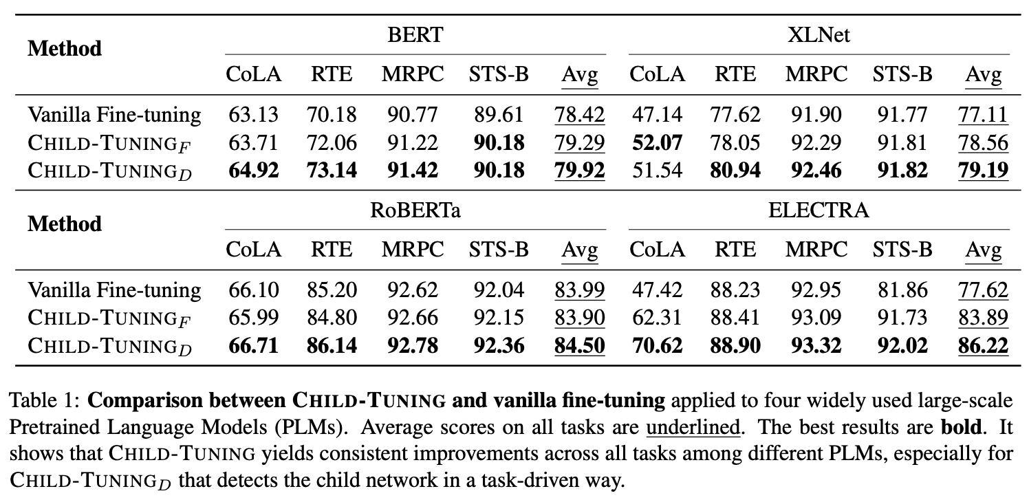ChildTuning results-1

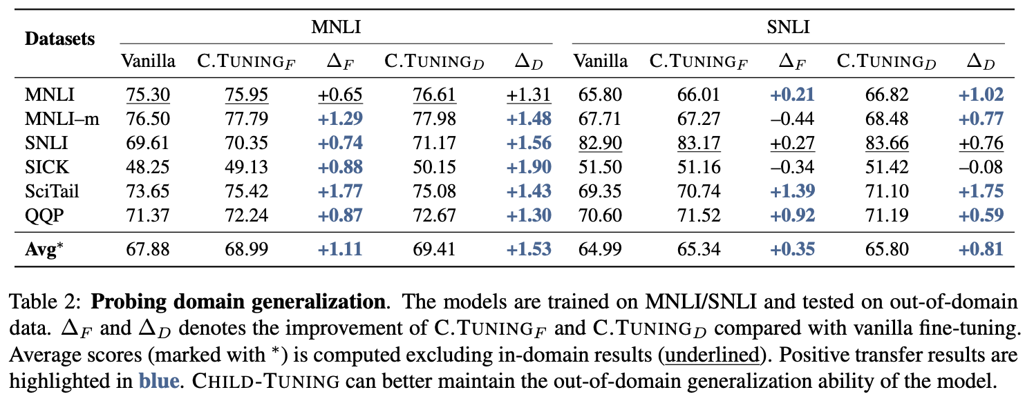ChildTuning results-2

From the tables, we can see that ChildTuning-D achieves improvements on almost all tasks, while ChildTuning-F is effective on quite a few tasks as well. Also, according to the paper's description, these are all results for the large version of the models; when I discussed this privately with the authors, they mentioned that the base version also shows improvements, but these weren't included in the paper due to space constraints.

Thinking About the Mechanism

ChildTuning-D ranks parameters based on Fisher information, an idea with a long history, so its effectiveness isn't particularly surprising — similar work includes Training Neural Networks with Fixed Sparse Masks, among others. What's more intriguing is that the task-independent ChildTuning-F, i.e. gradient Dropout, also turns out to work — this is worth thinking through carefully.

Coincidentally, there was another paper last year on applying Dropout to gradients, called Regularizing Meta-Learning via Gradient Dropout. This suggests that gradient Dropout probably does have some genuine effect. So why exactly does it work?

The Paper's Derivation

The original paper offers an SGD-based explanation, arguing that gradient Dropout enlarges the variance of the update process, which helps the model escape poor local optima.

Specifically, since we're using SGD, the gradient computed at each step has some inherent randomness; suppose it follows a Gaussian distribution with mean $\mu$ and variance $\sigma^2$. For ChildTuning-F, we introduce a random variable $\varepsilon$ that equals 1 with probability $p$, and 0 with the remaining probability $1-p$. Then we have

\begin{equation}\begin{aligned}&\mathbb{E}[g\varepsilon/p]=\mathbb{E}[g]\mathbb{E}[\varepsilon]/p=\mu \\ &\mathbb{E}[(g\varepsilon/p)^2]=\mathbb{E}[g^2]\mathbb{E}[\varepsilon^2]/p^2 = (\mu^2+\sigma^2)/p \end{aligned}\end{equation}

so

\begin{equation}\mathbb{V}ar[g\varepsilon/p] = \mathbb{E}[(g\varepsilon/p)^2] - \mathbb{E}[g\varepsilon/p]^2=\sigma^2 + \frac{1-p}{p}(\mu^2+\sigma^2) > \sigma^2\end{equation}

In other words, gradient Dropout keeps the mean of the gradient unchanged but enlarges its variance, and since in SGD the update is proportional to the gradient, gradient Dropout enlarges the variance of the update as well. The paper argues that this helps the model reach a better convergence point.

Answering a Different Question

This explanation looks quite reasonable at first glance, and it matches many people's intuitions, since many of us subconsciously believe that the reason stochastic gradient descent outperforms full-batch gradient descent is precisely the presence of noise. However, with just a bit more thought, we can see that the explanation above actually answers a different question than the one being asked.

The reason is simple: the analysis above is for SGD, but in practice, in NLP we almost always use Adam (or some variant of it). Does the above conclusion still hold for Adam? Unfortunately, no — in fact, it's exactly the opposite. In Adam, over the long run, the update can be approximated as (where $\eta$ is the learning rate)

\begin{equation}\Delta\theta = \eta\frac{\mathbb{E}[g]}{\sqrt{\mathbb{E}[g^2]}}\end{equation}

After adding gradient Dropout, the update becomes

\begin{equation}\eta\frac{\mathbb{E}[g\varepsilon/p]}{\sqrt{\mathbb{E}[(g\varepsilon/p)^2]}}=\eta\sqrt{p}\frac{\mathbb{E}[g]}{\sqrt{\mathbb{E}[g^2]}}\end{equation}

As you can see, over the long run, adding gradient Dropout to Adam is equivalent merely to shrinking the learning rate by a factor of $\sqrt{p}$! And because the learning rate — that is, the magnitude of the update — is reduced, the variance of the update is reduced accordingly as well. In other words, if you're using the Adam optimizer, the actual situation is the opposite of what the paper describes: the variance of the update doesn't increase at all, but decreases instead.

The fundamental reason for this phenomenon is that once we use an optimizer with a running average (momentum), the update is generally no longer proportional to the gradient. So how the gradient changes and how the update changes are not necessarily linked. This brings us back to my earlier question: why didn't the authors simply apply Dropout directly to the update instead? If it were update-level Dropout, then the SGD-based derivation above could actually be carried over directly.

My Own Interpretation

That said, I believe that even if we restrict ourselves to SGD, or apply Dropout directly to the update, the original paper's derivation still doesn't fully explain its effectiveness. The reason is simple: there are countless operations that could achieve "unchanged mean, enlarged variance" — for instance, simply adding some Gaussian noise directly to the gradient would also do this. Surely not all such operations would achieve the same effect? Personally, I find that unlikely. I believe that to explain the effectiveness of gradient Dropout or update Dropout, we need to focus on the sparsity that Dropout introduces.

On this point, I'm reminded of an earlier post I wrote, A Dynamical Systems Perspective on Optimization Algorithms (VII): SGD ≈ SVM?, which shows that any model trained via SGD ends up with a solution that is essentially SVM-like in form:

\begin{equation}f_{\theta_T}(x) = \beta(x) + \sum_i \alpha_i (x) K(x, x_i)\end{equation}

where $x_i$ is the $i$-th training sample. What's notable about this? $K(x,x_i)$ behaves like a "similarity function," and this form implies that the model effectively "memorizes" the training set in some sense, and then at prediction time retrieves from the training set using $K(x,x_i)$ as a similarity measure, producing a prediction accordingly. Of course, this is only a principled explanation — we don't deliberately design the model to take this form; rather, we're observing from this angle that gradient descent is in effect also memorizing samples, and producing predictions in a manner similar to KNN. This makes it easy to understand why, generally speaking, "more training samples lead to better results."

Coming back to ChildTuning-F: each time we sample a batch and apply Dropout to the computed gradient or update, combined with the "memorizing samples" interpretation above, we can intuitively picture this as "using only a small subset of parameters to memorize a small subset of samples," rather than always using the full set of parameters to memorize that same small batch. So this should be analogous to the principle of "not putting all your eggs in one basket" — by spreading the samples more evenly across the parameters, the risk of overfitting is reduced.

Giving It a Try

For ChildTuning-F, if you're comfortable modifying the optimizer yourself, whether you apply Dropout to the gradient or to the update, it's really just a one-line change, so it's worth experimenting with. Who knows — maybe it actually helps!

Here I ran some tests on several CLUE tasks; the results are shown in the table below. The baseline code comes from bert4keras in Hand, I've Got the Baseline: CLUE Benchmark Code. "grad drop" refers to applying Dropout to the gradient, "incre drop" refers to applying Dropout to the update; green indicates an improvement over the baseline, and red indicates a decline. Given limited time and compute, all results were run only once, so there's some inherent random fluctuation.

$$\begin{array}{c} \text{CLUE classification comparison (val set)} \\ {\begin{array}{c|ccccccc} \hline & \text{IFLYTEK} & \text{TNEWS} & \text{AFQMC} & \text{OCNLI} & \text{CMNLI} & \text{WSC} & \text{CSL} \\ \hline \text{BERT} & 60.06 & 56.80 & 72.41 & 73.93 & 79.56 & 78.62 & 83.93 \\ \text{BERT}_{\text{-grad drop}} & \color{green}{60.56} & \color{green}{56.97} & \color{red}{72.13} & \color{green}{74.88} & \color{green}{80.09} & \color{red}{75.99} & \color{red}{83.83} \\ \text{BERT}_{\text{-incre drop}} & \color{red}{59.99} & \color{red}{56.78} & \color{green}{72.66} & \color{green}{74.51} & \color{red}{79.36} & \color{red}{77.30} & \color{green}{84.20} \\ \hline \text{RoBERTa} & 60.64 & 58.06 & 74.05 & 76.00 & 81.24 & 87.50 & 84.50\\ \text{RoBERTa}_{\text{-grad drop}} & \color{green}{60.72} & \color{red}{57.91} & \color{red}{74.03} & \color{red}{75.19} & \color{red}{80.52} & \color{red}{84.54} & \color{green}{84.73}\\ \text{RoBERTa}_{\text{-incre drop}} & \color{green}{60.87} & \color{red}{57.99} & \color{red}{74.03} & \color{red}{75.97} & \color{red}{81.02} & \color{red}{84.87} & \color{green}{84.73}\\ \hline \end{array}} \end{array}$$

From the table, we can roughly conclude:

1. Applying Dropout to the gradient versus applying it to the update each has its own pros and cons, more or less;
2. The effect is more noticeable on BERT, and almost nonexistent on RoBERTa — this is consistent with the English-language experimental results reported in the paper.

This result is honestly a bit frustrating. It's not that it doesn't work, but realistically, who would choose to use BERT — which runs at the same speed but performs worse — over RoBERTa, which performs better? So if it doesn't really work on RoBERTa, does it seem like there's not much point in trying it at all? Of course, the biggest improvement in the original paper was on Electra, which I haven't tried myself — if any interested readers give it a shot, please let me know the results.

Also, I don't have a particular interest in ChildTuning-D, and its implementation is a bit more involved, so I didn't experiment with it. Readers who have tried it are welcome to share their results too.

Summary

This post introduced the idea of adding Dropout to gradients to improve fine-tuning performance, along with my own theoretical analysis. Overall, my take is: it's worth trying, it might work, but don't set your expectations too high.