Dropout Twice Again! This Time It Achieves SOTA on Supervised Tasks

又是Dropout两次！这次它做到了有监督任务的SOTA 苏剑林 · 2021-07-01 · Machine Learning optimization loss function adversarial training

Readers keeping up with recent NLP developments will surely remember SimCSE, released in April, which constructs positive pairs for contrastive learning through the simple trick of "applying Dropout twice," achieving an across-the-board SOTA on unsupervised semantic similarity tasks. Coincidentally, a recent paper, R-Drop: Regularized Dropout for Neural Networks, proposes R-Drop, which applies the same "Dropout twice" idea to supervised tasks, obtaining a clear improvement in nearly every experiment. On top of that, in my own experiments I found that it also performs quite well on semi-supervised tasks.

It's rather remarkable that such a small trick as "Dropout twice" turns out to be a jack of all trades. In this post I'll introduce R-Drop and share my own thoughts on the reasoning behind it.

SimCSE

In Is It Still SOTA on Chinese Tasks? We Add Some Experiments to SimCSE, we already introduced SimCSE. In short, SimCSE is a contrastive learning scheme for NLP. The standard contrastive-learning pipeline treats the results obtained from the same sample via different data augmentation methods as a positive pair, while all other samples in the batch are treated as negatives; a loss function is then used to pull positive pairs closer together and push negative pairs farther apart.

So the main difficulty lies in the data augmentation method. For NLP, it's hard to manually construct augmentations that are guaranteed to preserve semantics, so SimCSE simply dispenses with manual data augmentation altogether, instead obtaining two different feature vectors for the same input by "applying Dropout twice," and treating these as a positive pair. Curiously, this simple "Dropout twice" trick for constructing positive pairs, which looks like a reluctant compromise, turns out in ablation studies to outperform almost every other data augmentation method — surprising, and yet also a reminder that "the great truth is often simple."

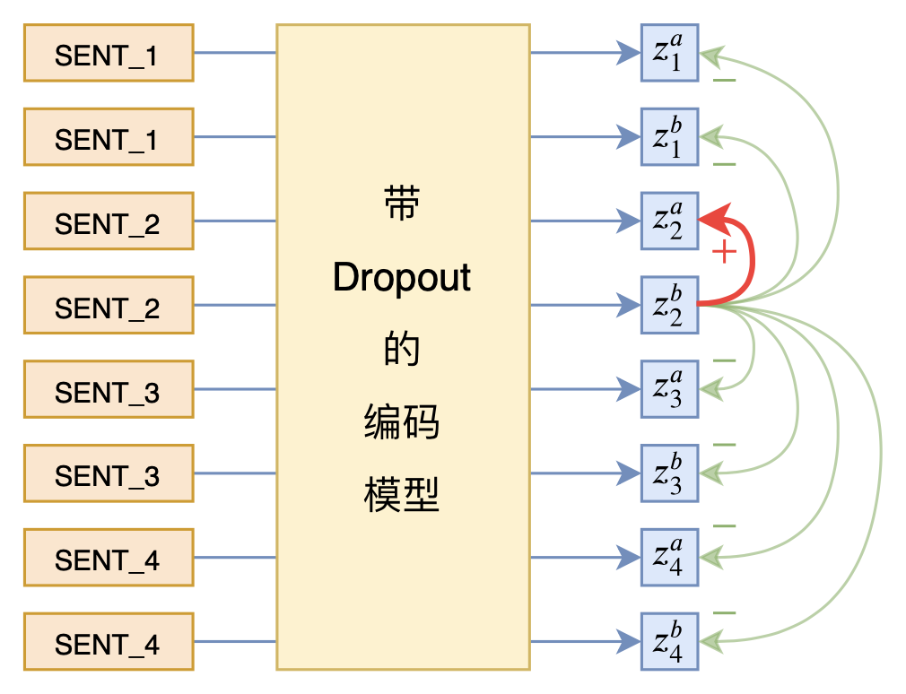SimCSE diagram

In terms of implementation, SimCSE is also remarkably simple. The so-called "Dropout twice" only requires feeding the same sample into the model twice and then computing the corresponding loss, as shown in the figure above. Because Dropout itself is random, each pass through the model applies a different Dropout mask, so simply duplicating the sample is enough to achieve the "Dropout twice" effect.

R-Drop

Looking at the results, what SimCSE really wants is for Dropout to have little effect on the model's output — in other words, for the model's output to be robust to Dropout. So it's clear that this "Dropout twice" idea can be generalized to tasks in general, and that's exactly what R-Drop (Regularized Dropout) does.

Classification Problems

In my view, R-Drop is highly related to SimCSE — I'd even guess R-Drop was inspired by SimCSE — yet the R-Drop paper doesn't cite SimCSE at all, which is a bit puzzling.

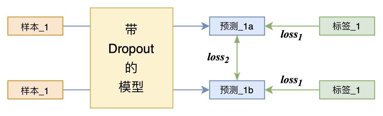R-Drop diagram

Concretely, take classification as an example. The training data is $\{x_i,y_i\}_{i=1}^n$, the model is $P_{\theta}(y|x)$, and the loss for each sample is generally the cross-entropy

\begin{equation}\mathcal{L}_i = -\log P_{\theta}(y_i|x_i)\end{equation}

Under "Dropout twice," we can think of the sample as having passed through two slightly different models, which we denote $P_{\theta}^{(1)}(y|x)$ and $P_{\theta}^{(2)}(y|x)$. The R-Drop loss then has two parts. One is the usual cross-entropy:

\begin{equation}\mathcal{L}_i^{(CE)} = -\log P_{\theta}^{(1)}(y_i|x_i) -\log P_{\theta}^{(2)}(y_i|x_i)\label{eq:ce}\end{equation}

The other is the symmetric KL divergence between the two models, which encourages the outputs under different Dropout masks to be as consistent as possible:

\begin{equation}\mathcal{L}_i^{(KL)} = \frac{1}{2}\big[KL\left(P_{\theta}^{(2)}(y|x_i)\big\Vert P_{\theta}^{(1)}(y|x_i)\right) + KL\left(P_{\theta}^{(1)}(y|x_i)\big\Vert P_{\theta}^{(2)}(y|x_i)\right)\big]\label{eq:kl}\end{equation}

The final loss is a weighted sum of the two:

\begin{equation}\mathcal{L}_i = \mathcal{L}_i^{(CE)} + \alpha\mathcal{L}_i^{(KL)}\end{equation}

In other words, on top of the ordinary cross-entropy, a regularization term is added that reinforces the model's robustness.

General Form

Some readers might ask what to substitute for the $KL$ term in non-classification problems. In fact the original paper doesn't run experiments on non-classification tasks, but we can fill that gap here. Notice that

\begin{equation}-\log P_{\theta}(y_i|x_i) = KL\left(\text{one_hot}(y_i)\big\Vert P_{\theta}(y|x_i)\right)\end{equation}

so the $\mathcal{L}_i$ term above is really just a repeated application of the $KL$ divergence, and its general form is:

\begin{equation}\mathcal{L}_i = \mathcal{D}\left(y_i, f_{\theta}^{(1)}(x_i)\right)+\mathcal{D}\left(y_i, f_{\theta}^{(2)}(x_i)\right) + \frac{\alpha}{2} \left[\mathcal{D}\left(f_{\theta}^{(2)}(x_i), f_{\theta}^{(1)}(x_i)\right)+\mathcal{D}\left(f_{\theta}^{(1)}(x_i), f_{\theta}^{(2)}(x_i)\right)\right]\end{equation}

Hence, for non-classification tasks we simply replace $\mathcal{D}$ with an appropriate measure (rather than the $KL$ divergence).

Experimental Results

Let's first look at R-Drop's experimental results.

R-Drop has three main hyperparameters: batch size, $\alpha$, and the Dropout probability. Batch size is generally dictated by our available compute, so there's not much room to tune it individually; the original paper tries $\alpha$ ranging over $1\sim 5$, while in my own experiments I simply used $\alpha=4$ without fine-tuning it. As for the Dropout probability, following the same choice as in Is It Still SOTA on Chinese Tasks? We Add Some Experiments to SimCSE, setting it to 0.3 works reasonably well.

Results Reported in the Paper

Honestly, the results reported for R-Drop in the original paper are quite impressive, and that's the main reason I felt compelled to write this introduction. The paper runs comparative experiments on R-Drop across various NLU, NLG, and CV classification tasks, and most of them show a "clear improvement."

Official implementation: https://github.com/dropreg/R-Drop

Here are some screenshots of the experimental results:

R-Drop's effect on machine translation tasks

R-Drop's effect on GLUE tasks

In particular, on machine translation, plain "Transformer + R-Drop" surpasses more complex alternative methods:

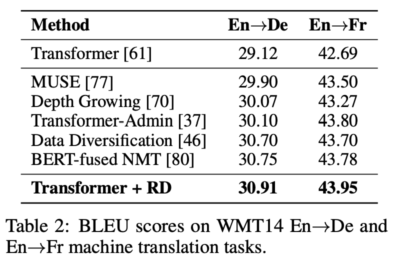Comparison of different methods on machine translation

The paper also includes experiments on summarization, language modeling, image classification, and some ablations over hyperparameters, which I encourage readers to check out in the original paper. All in all, this "report card" for R-Drop is impressive enough to deserve applause.

My Own Experiments

Of course, I stand by the view that "a model that hasn't been tested on Chinese has no soul," so I generally only write about something after I've personally tried it on a Chinese task.

My own implementation: https://github.com/bojone/r-drop

For Chinese supervised tasks, I tried two text classification tasks (IFLYTEK and TNEWS from the CLUE benchmark)

$$\begin{array}{c|cc} \hline & \text{IFLYTEK} & \text{TNEWS} \\ \hline \text{no adversarial training} & 60.29\% & 56.58\% \\ \text{add adversarial training} & 62.46\% & 57.66\% \\ \text{add gradient penalty} & 62.31\% & \textbf{57.81%} \\ \text{add R-Drop} & \textbf{62.69%} & 57.51\% \\ \hline \end{array}$$

and one text generation task (CSL title generation, referring to A Brief Analysis of and Countermeasures for Exposure Bias in Seq2Seq):

$$\begin{array}{c|cccc} \hline & \text{Rouge-L} & \text{Rouge-1} & \text{Rouge-2} & \text{BLEU} \\ \hline \text{baseline} & 63.81 & 65.45 & 54.91 & 45.52 \\ \text{random replace} & 64.44 & 66.09 & 55.56 & 46.1 \\ \text{gradient penalty} & 65.41 & 67.29 & 56.64 & 47.37 \\ \text{R-Drop} & \textbf{65.51} & \textbf{67.41} & \textbf{57.12} & \textbf{47.82} \\ \hline \end{array}$$

As you can see, R-Drop's results are strong enough to compete with the famous regularization methods "adversarial training" and "gradient penalty" introduced in A Brief Discussion of Adversarial Training: Meaning, Methods, and Reflections (with Keras Implementation).

Implementation Notes

Compared with more complex regularization methods like adversarial training, R-Drop is remarkably easy to implement. Here I'll use bert4keras as an example to briefly show how to turn an ordinary training script into a Dropout-twice version.

First, here's the change to the data generator:

class data_generator(DataGenerator):
    """数据生成器
    """
    def __iter__(self, random=False):
        batch_token_ids, batch_segment_ids, batch_labels = [], [], []
        for is_end, (text, label) in self.sample(random):
            token_ids, segment_ids = tokenizer.encode(text, maxlen=maxlen)
            # batch_token_ids.append(token_ids)
            # batch_segment_ids.append(segment_ids)
            # batch_labels.append([label])
            for i in range(2):
                batch_token_ids.append(token_ids)
                batch_segment_ids.append(segment_ids)
                batch_labels.append([label])
            # if len(batch_token_ids) == self.batch_size or is_end:
            if len(batch_token_ids) == self.batch_size * 2 or is_end:
                batch_token_ids = sequence_padding(batch_token_ids)
                batch_segment_ids = sequence_padding(batch_segment_ids)
                batch_labels = sequence_padding(batch_labels)
                yield [batch_token_ids, batch_segment_ids], batch_labels
                batch_token_ids, batch_segment_ids, batch_labels = [], [], []

Then, define a new custom loss:

from keras.losses import kullback_leibler_divergence as kld

def categorical_crossentropy_with_rdrop(y_true, y_pred):
    """配合上述生成器的R-Drop Loss
    其实loss_kl的除以4，是为了在数量上对齐公式描述结果。
    """
    loss_ce = K.categorical_crossentropy(y_true, y_pred)  # 原来的loss
    loss_kl = kld(y_pred[::2], y_pred[1::2]) + kld(y_pred[1::2], y_pred[::2])
    return K.mean(loss_ce) + K.mean(loss_kl) / 4 * alpha

Finally, turn on Dropout in the model, and train it using this data_generator and categorical_crossentropy_with_rdrop.

My Own Understanding

Having enjoyed these pleasing experimental results, let's dig into the theory. The original paper offers a theoretical analysis of R-Drop, roughly arguing that R-Drop promotes parameter assimilation, thereby acting as a regularizer. Personally, though, I don't find this explanation very intuitive, nor does it get at the essence of the matter. Below I'll try to offer a few alternative angles for understanding R-Drop.

Consistency

R-Drop can be seen as an improvement on Dropout — so what's wrong with plain Dropout? The issue is that Dropout is a classic example of a train/test mismatch. Specifically, during training Dropout adds multiplicative noise to the input (of certain layers), turning the model from $f_{\theta}(x)$ into $f_{\theta}(x,\varepsilon)$, where each element of $\varepsilon$ is 0 with probability $p$ and otherwise takes the value $1/(1-p)$ with probability $1-p$. The training objective is then

\begin{equation}\mathbb{E}_{(x,y)\sim\mathcal{D}}\mathbb{E}_{\varepsilon}[l(y, f_{\theta}(x,\varepsilon))]\end{equation}

Once trained this way, which model should we actually use for prediction? It's not obvious — but if the loss function is the $l_2$ distance, we can show that the optimal prediction model should be

\begin{equation}\mathbb{E}_{\varepsilon}[f_{\theta}(x,\varepsilon)]\end{equation}

Derivation:
If we use the $l_2$ loss, the loss for a single sample is
\begin{equation}\mathbb{E}_{\varepsilon}\left[\Vert y - f_{\theta}(x,\varepsilon)\Vert^2\right] = \Vert y\Vert^2 - 2\langle y,\mathbb{E}_{\varepsilon}\left[f_{\theta}(x,\varepsilon)\right]\rangle + \mathbb{E}_{\varepsilon}\left[\Vert f_{\theta}(x,\varepsilon)\Vert^2\right]\end{equation}
Note that our question here is "what function should we use for prediction once training is finished," so $f_{\theta}(x,\varepsilon)$ is fixed while $y$ is the variable we're optimizing over. This is simply minimizing a quadratic function, and it's easy to see the minimum is achieved when $y=\mathbb{E}_{\varepsilon}[f_{\theta}(x,\varepsilon)]$.

We'll assume this result generalizes to the general case. The equation above tells us that the correct way to use a model trained with Dropout is via "model averaging":

Pass the same input through the model multiple times (without turning off Dropout), and average the multiple predictions to get the final prediction.

But this is clearly not how we typically make predictions in practice — instead, we simply turn off Dropout and make a deterministic prediction. This effectively switches the prediction model from "averaging models" to "averaging weights":

\begin{equation}f_{\theta}(x,\mathbb{E}_{\varepsilon}[\varepsilon])=f_{\theta}(x,1)=f_{\theta}(x)\end{equation}

Here $1$ denotes the all-ones vector. So during training we're effectively training an ensemble over different Dropout masks, but at test time we use a single model with Dropout turned off — the two are not necessarily equivalent, and this is exactly the train/test inconsistency problem of Dropout.

Now it's easy to see what R-Drop is doing: by adding a regularization term, it strengthens the model's robustness to Dropout, making the outputs under different Dropout masks essentially consistent. This reduces the inconsistency described above and makes "model averaging" and "weight averaging" more similar to each other — so that simply turning off Dropout at test time becomes equivalent to ensembling over many Dropout-perturbed models, ultimately improving the model's final performance.

Continuity

At the very beginning of this post I mentioned the similarity between R-Drop and SimCSE. In fact, R-Drop is also quite similar to another method: Virtual Adversarial Training (VAT). (And yet R-Drop doesn't cite VAT either — am I the only one who sees the resemblance??)

For an introduction to VAT, see my earlier post Random Musings on Generalization: From Random Noise and Gradient Penalty to Virtual Adversarial Training. In short, VAT also uses a regularization term to make the model more robust to perturbations, enhancing the model's own continuity (so that small changes don't cause large changes in the output). The difference lies in how the perturbation is applied: VAT only perturbs the input, and uses adversarial optimization to make the perturbation as targeted as possible; R-Drop's perturbation, on the other hand, can be applied to every layer of the model, and it is random rather than adversarially optimized.

Some readers may already be thinking: VAT is well known for semi-supervised training, so does that mean R-Drop can also be used for semi-supervised training? The original paper doesn't run this experiment — I did it myself — and the answer is yes, it works. Like VAT, R-Drop's added KL divergence term doesn't require labels, so it can be trained unsupervised; mixing it with supervised training gives semi-supervised training, and the results are quite good. Here are my experimental results:

$$\begin{array}{c|cc} \hline & \text{val set} & \text{test set}\\ \hline \text{non-VAT} & 88.93\% & 89.34\%\\ \text{VAT} & 89.83\% & \textbf{90.37%}\\ \text{R-Drop} & \textbf{90.37%} & 90.14\%\\ \hline \end{array}$$

As you can see, R-Drop's performance in the semi-supervised setting is entirely on par with VAT, and it's simpler to implement and faster to run than VAT! It looks like VAT might be ready for retirement. Intuitively, although R-Drop's perturbations are random, there are more of them, so their overall effect gets amplified, which may let them rival the perturbations that VAT carefully optimizes adversarially — which is likely why R-Drop can match VAT's performance.

Non-Target Classes

A fairly direct question is: if my model is complex enough, can't cross-entropy alone make the model robust to Dropout? What concrete difference does the KL divergence term actually make?

As it turns out, no, it really can't. The key point is that the training objective of cross-entropy is essentially: make the score of the target class higher than the scores of the non-target classes, so that the model can correctly predict the target class (see Generalizing "Softmax + Cross-Entropy" to Multi-Label Classification). In other words, if we only use cross-entropy, the most the model's training can achieve is:

Under different Dropout masks, the target class's score is always higher than the non-target classes' scores

but it cannot achieve:

Under different Dropout masks, the score of every class stays consistent

So the train/test inconsistency problem is not actually solved. Looking at the formula, the cross-entropy $\eqref{eq:ce}$ only depends on the target class and ignores the distribution over non-target classes — if the target class is the first class, then predictions of $[0.5, 0.2, 0.3]$ and $[0.5, 0.3, 0.2]$ make no difference to it. But for the KL divergence term $\eqref{eq:kl}$, things are different: every class's score participates in the computation, and $[0.5, 0.2, 0.3]$ versus $[0.5, 0.3, 0.2]$ will incur a nonzero loss.

Summary

This post introduced R-Drop, which applies the "Dropout twice" idea to supervised tasks, achieving a clear improvement in nearly every experiment. In addition, I found in my own experiments that it also performs quite well on semi-supervised tasks. Finally, I shared three different angles for thinking about why R-Drop works.