A Brief Introduction to Adversarial Training: Meaning, Methods, and Reflections (with Keras Implementation)
Currently, when talking about "adversarial" in deep learning, there are generally two meanings: one is Generative Adversarial Networks (GAN), which represents a broad class of advanced generative models; the other is the field related to adversarial attacks and adversarial examples. This is related to GANs but quite different, and it is mainly concerned with the robustness of models under small perturbations. The adversarial topics covered previously on this blog have all been about the first meaning, but today we're going to talk about "adversarial training" in the sense of the second meaning.
This post covers the following:
1. An introduction to basic concepts such as adversarial examples and adversarial training;
2. An introduction to adversarial training based on fast gradient ascent and its applications in NLP;
3. A Keras implementation of adversarial training (callable with one line of code);
4. A discussion of the equivalence between adversarial training and gradient penalty;
5. Based on gradient penalty, an intuitive geometric understanding of adversarial training.
Method Overview
In recent years, with the growing development and deployment of deep learning, adversarial examples have received increasing attention. In the CV field, we need to strengthen model robustness through adversarial attacks and defenses—for example, in autonomous driving systems, we need to prevent the model from misidentifying a red light as a green light due to some random noise. Similar adversarial training also exists in the NLP field, but adversarial training in NLP is more often used as a regularization technique to improve the model's generalization ability!
This has made adversarial training one of the "secret weapons" for climbing NLP leaderboards. Microsoft previously used RoBERTa + adversarial training to surpass the original RoBERTa on the GLUE leaderboard, and colleagues at my company later used adversarial training to set a new record on the CoQA leaderboard. This successfully piqued my interest, so I studied it a bit and I'm sharing what I learned here.
Basic Concepts
To understand adversarial training, we first need to understand "adversarial examples," which first appeared in the paper Intriguing properties of neural networks. Simply put, these are samples that "look" almost identical to humans but produce completely different predictions from the model. Consider the classic example below:
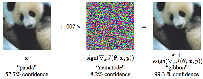 A classic adversarial example, from the paper "Explaining and Harnessing Adversarial Examples"
Once you understand adversarial examples, it's not hard to understand the related concepts. "Adversarial attacks" refers to finding ways to construct more adversarial examples, while "adversarial defense" refers to finding ways to make the model correctly identify more adversarial examples. So-called adversarial training is a type of adversarial defense: it constructs some adversarial examples and adds them to the original dataset, hoping to enhance the model's robustness to adversarial examples. At the same time, as mentioned at the beginning of this post, in NLP it can often also improve model performance.
Min-Max
In general, adversarial training can be written uniformly as follows:
\begin{equation}\min_{\theta}\mathbb{E}_{(x,y)\sim\mathcal{D}}\left[\max_{\Delta x\in\Omega}L(x+\Delta x, y;\theta)\right]\label{eq:min-max}\end{equation}
Here $\mathcal{D}$ denotes the training set, $x$ the input, $y$ the label, $\theta$ the model parameters, $L(x,y;\theta)$ the loss for a single sample, $\Delta x$ the adversarial perturbation, and $\Omega$ the perturbation space. This unified formulation was first proposed in the paper Towards Deep Learning Models Resistant to Adversarial Attacks.
This expression can be understood step by step as follows:
1. We inject a perturbation $\Delta x$ into $x$; the goal of $\Delta x$ is to make $L(x+\Delta x, y;\theta)$ as large as possible, i.e., to make the current model's predictions go as wrong as possible;
2. Of course, $\Delta x$ is not unconstrained—it can't be too large, otherwise it wouldn't achieve the effect of "looking almost the same." So $\Delta x$ must satisfy certain constraints, typically $\Vert\Delta x\Vert\leq \epsilon$, where $\epsilon$ is a constant;
3. After constructing the adversarial example $x+\Delta x$ for each sample, we use $(x + \Delta x, y)$ as the data pair to minimize the loss and update the parameters $\theta$ (gradient descent);
4. Steps 1, 2, and 3 are repeated alternately.
From this we can see that the whole optimization process alternates between $\max$ and $\min$, which indeed resembles GANs quite closely. The difference is that in GANs, the variable being $\max$'d over is also the model parameters, whereas here the variable being $\max$'d over is the input (its perturbation)—that is, we need to customize one step of $\max$ for every single input.
Fast Gradient
Now the question is how to compute $\Delta x$. Its goal is to increase $L(x+\Delta, y;\theta)$, and we know that the way to decrease a loss is gradient descent, so conversely, the way to increase a loss is naturally gradient ascent. So we can simply take
\begin{equation}\Delta x = \epsilon \nabla_x L(x, y;\theta)\end{equation}
Of course, to prevent $\Delta x$ from becoming too large, we usually need to normalize $\nabla_x L(x, y;\theta)$ in some way, and a common approach is
\begin{equation}\Delta x = \epsilon \frac{\nabla_x L(x, y;\theta)}{\Vert \nabla_x L(x, y;\theta)\Vert}\quad\text{or}\quad \Delta x = \epsilon \text{sign}(\nabla_x L(x, y;\theta))\end{equation}
Once we have $\Delta x$, we can substitute it back into formula $\eqref{eq:min-max}$ to perform the optimization:
\begin{equation}\min_{\theta}\mathbb{E}_{(x,y)\sim\mathcal{D}}\left[L(x+\Delta x, y;\theta)\right]\end{equation}
This constitutes an adversarial training method known as the Fast Gradient Method (FGM), first proposed by Goodfellow, the father of GANs, in the paper Explaining and Harnessing Adversarial Examples.
In addition, there is another adversarial training method called Projected Gradient Descent (PGD), which essentially achieves a larger increase in $L(x+\Delta x,y;\theta)$ for $\Delta x$ by iterating several more steps (if the norm exceeds $\epsilon$ during the iteration, it is scaled back down; for details, please refer to Towards Deep Learning Models Resistant to Adversarial Attacks). However, this post does not aim to give a complete introduction to adversarial learning, and I personally feel PGD is not as elegant or effective as FGM, so this post will focus on FGM. For a supplementary introduction to adversarial training, interested readers are encouraged to read the post by Fubang, Attack and Defense: Adversarial Training in NLP + PyTorch Implementation.
Back to NLP
For tasks in the CV domain, the adversarial training procedure described above can be carried out smoothly, because images can be treated as ordinary continuous real-valued vectors, and $\Delta x$ is also a real-valued vector, so $x+\Delta x$ can still be a meaningful image. But NLP is different: the input to NLP is text, which is essentially a one-hot vector (if you haven't yet realized this, feel free to read What Exactly Are Word Embeddings?), and the Euclidean distance between two distinct one-hot vectors is always $\sqrt{2}$. So in theory, there is no such thing as a "small perturbation" here.
A natural idea, following the paper Adversarial Training Methods for Semi-Supervised Text Classification, is to add the perturbation to the embedding layer. There's no problem with this approach operationally, but the issue is that a perturbed embedding vector doesn't necessarily correspond to any entry in the original embedding table. This means the perturbation on the embedding layer no longer corresponds to a real text input, so it's no longer a genuine adversarial example in the proper sense—since an adversarial example should still correspond to a valid original input.
So does perturbing the embedding layer even make sense, then? Yes! Experimental results show that in many tasks, adversarial perturbation at the embedding layer can effectively improve model performance.
Experimental Results
Since it works, we naturally want to verify it ourselves. How do we implement adversarial training in code? How do we make it as simple as possible to use? And what results do we actually get?
Approach
For CV tasks, the input tensor shape is typically $(b,h,w,c)$. In this case, we need to fix the model's batch size (i.e., $b$), and then add to the original input a zero-initialized Variable of the same shape $(b,h,w,c)$, let's call it $\Delta x$. We can then directly compute the gradient of the loss with respect to $x$, and assign a value to $\Delta x$ based on that gradient to perturb the input. After applying the perturbation, we proceed with regular gradient descent.
For NLP tasks, in principle we should do the same thing at the output of the embedding layer. The output shape of the embedding layer is $(b,n,d)$, so we would also need to add a Variable of shape $(b,n,d)$ to the embedding layer's output, and then carry out the steps above. But this would require decomposing and reconstructing the model, which is not very user-friendly.
However, we can settle for a slightly less ideal approach. The output of the embedding layer is taken directly from the embedding parameter matrix, so we can directly perturb the embedding parameter matrix itself. The adversarial examples obtained this way will have somewhat less diversity (since the same token across different samples shares the same perturbation), but this still serves a regularizing purpose, and it's much easier to implement.
Reference Code
Based on the approach above, here is a reference implementation in Keras of FGM-style adversarial training on the embedding layer:
https://github.com/bojone/keras_adversarial_training
The core code is as follows:
def adversarial_training(model, embedding_name, epsilon=1):
    """给模型添加对抗训练
    其中model是需要添加对抗训练的keras模型,embedding_name
    则是model里边Embedding层的名字。要在模型compile之后使用。
    """
    if model.train_function is None:  # 如果还没有训练函数
        model._make_train_function()  # 手动make
    old_train_function = model.train_function  # 备份旧的训练函数

    # 查找Embedding层
    for output in model.outputs:
        embedding_layer = search_layer(output, embedding_name)
        if embedding_layer is not None:
            break
    if embedding_layer is None:
        raise Exception('Embedding layer not found')

    # 求Embedding梯度
    embeddings = embedding_layer.embeddings  # Embedding矩阵
    gradients = K.gradients(model.total_loss, [embeddings])  # Embedding梯度
    gradients = K.zeros_like(embeddings) + gradients[0]  # 转为dense tensor

    # 封装为函数
    inputs = (model._feed_inputs +
              model._feed_targets +
              model._feed_sample_weights)  # 所有输入层
    embedding_gradients = K.function(
        inputs=inputs,
        outputs=[gradients],
        name='embedding_gradients',
    )  # 封装为函数

    def train_function(inputs):  # 重新定义训练函数
        grads = embedding_gradients(inputs)[0]  # Embedding梯度
        delta = epsilon * grads / (np.sqrt((grads**2).sum()) + 1e-8)  # 计算扰动
        K.set_value(embeddings, K.eval(embeddings) + delta)  # 注入扰动
        outputs = old_train_function(inputs)  # 梯度下降
        K.set_value(embeddings, K.eval(embeddings) - delta)  # 删除扰动
        return outputs

    model.train_function = train_function  # 覆盖原训练函数
Once the function above is defined, adding adversarial training to a Keras model requires just one line of code:
# 写好函数后,启用对抗训练只需要一行代码
adversarial_training(model, 'Embedding-Token', 0.5)
It should be noted that since computing the adversarial perturbation at each step also requires computing a gradient, each training step now involves two gradient computations, so the training time per step roughly doubles.
Performance Comparison
To test the practical effect, I selected two classification tasks from the Chinese CLUE leaderboard: IFLYTEK and TNEWS, using the Chinese BERT-base model. On the CLUE leaderboard, BERT-base's scores on these two datasets are 60.29% and 56.58% respectively. After adversarial training, the scores became 62.46% and 57.66%—improvements of about 2% and 1% respectively!
$$\begin{array}{c|cc} \hline & \text{IFLYTEK} & \text{TNEWS} \\ \hline \text{no adversarial training} & 60.29\% & 56.58\% \\ \text{add adversarial training} & 62.46\% & 57.66\% \\ \hline \end{array}$$
Please refer to the training script here: task_iflytek_adversarial_training.py.
Of course, like all regularization techniques, adversarial training can't guarantee improvement on every single task, but judging from the results reported so far, it's a technique well worth trying. Also, fine-tuning BERT itself is already a rather mysterious process that depends a lot on luck—not long ago, the paper Fine-Tuning Pretrained Language Models: Weight Initializations, Data Orders, and Early Stopping ran hundreds of fine-tuning experiments with different random seeds and found that the best result could be several points higher than average. So if you run it once and see no improvement, it might be worth running it a few more times before drawing conclusions.
Further Reflections
In this section, we'll analyze the above results from another angle, which will lead us to another method of adversarial training, and give us a more intuitive geometric understanding of adversarial training.
Gradient Penalty
Suppose we've already obtained the adversarial perturbation $\Delta x$. Then, when updating $\theta$, consider the expansion of $L(x+\Delta x, y;\theta)$:
\begin{equation}\begin{aligned}&\min_{\theta}\mathbb{E}_{(x,y)\sim\mathcal{D}}\left[L(x+\Delta x, y;\theta)\right]\\ \approx&\, \min_{\theta}\mathbb{E}_{(x,y)\sim\mathcal{D}}\left[L(x, y;\theta)+\langle\nabla_x L(x, y;\theta), \Delta x\rangle\right] \end{aligned}\end{equation}
The corresponding gradient with respect to $\theta$ is
\begin{equation}\nabla_{\theta}L(x, y;\theta)+\langle\nabla_{\theta}\nabla_x L(x, y;\theta), \Delta x\rangle\end{equation}
Substituting into $\Delta x=\epsilon \nabla_x L(x, y;\theta)$, we obtain
\begin{equation}\begin{aligned}&\nabla_{\theta}L(x, y;\theta)+\epsilon\langle\nabla_{\theta}\nabla_x L(x, y;\theta), \nabla_x L(x, y;\theta)\rangle\\ =&\,\nabla_{\theta}\left(L(x, y;\theta)+\frac{1}{2}\epsilon\left\Vert\nabla_x L(x, y;\theta)\right\Vert^2\right) \end{aligned}\end{equation}
This result tells us that applying an adversarial perturbation of magnitude $\epsilon \nabla_x L(x, y;\theta)$ to the input sample is, to some extent, equivalent to adding a "gradient penalty" to the loss:
\begin{equation}\frac{1}{2}\epsilon\left\Vert\nabla_x L(x, y;\theta)\right\Vert^2\label{eq:gp}\end{equation}
If the adversarial perturbation is $\epsilon \nabla_x L(x, y;\theta)/\Vert \nabla_x L(x, y;\theta)\Vert$, then the corresponding gradient penalty term is $\epsilon\left\Vert\nabla_x L(x, y;\theta)\right\Vert$ (missing a factor of $1/2$, and also missing the square).
In fact, this result isn't new—as far as I know, it first appeared in the paper Improving the Adversarial Robustness and Interpretability of Deep Neural Networks by Regularizing their Input Gradients. It's just that this paper isn't easy to find, because once you search for keywords like "adversarial training gradient penalty," almost all the results that come up are related to WGAN-GP.
Geometric Picture
In fact, there's a very intuitive geometric picture for gradient penalty. Take a standard classification problem as an example: suppose there are $n$ classes, so the model is essentially digging $n$ pits, and then putting samples of the same class into the same pit:
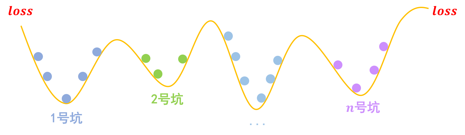 A classification problem is like digging pits, then placing samples of the same class into the same pit
Gradient penalty says: "Samples of the same class should not only be placed in the same pit, they should be placed at the bottom of the pit." This requires each pit to look like this internally:
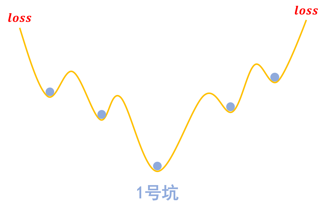 Adversarial training wants every sample to sit at the bottom of a "pit within a pit"
Why the bottom of the pit? Because physics tells us that the bottom of a pit is the most stable place, so it's the least susceptible to disturbance—and isn't that exactly the goal of adversarial training?
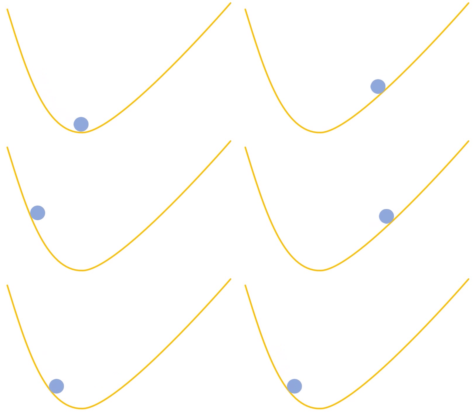 The "bottom of the pit" is the most stable. After being disturbed, the sample still lingers near the bottom and doesn't easily jump out of the pit (jumping out of the pit usually means misclassification)
So what does "the bottom of the pit" mean? It's a local minimum, where the derivative (gradient) is zero—so isn't this exactly the same as wanting $\Vert\nabla_x L(x,y;\theta)\Vert$ to be as small as possible? This is the geometric meaning of the gradient penalty $\eqref{eq:gp}$. For similar geometric pictures of "digging pits," "pit bottoms," and gradient penalty, you can also refer to GANs from an Energy Perspective (I): GAN = "Digging Pits" + "Jumping into Pits".
The L-Constraint
We can also look at gradient penalty from the perspective of the L-constraint (Lipschitz constraint). What is an adversarial example, if not a small perturbation of the input causing a large change in the output? We previously discussed the issue of controlling the relationship between input and output in the article The L-Constraint in Deep Learning: Generalization and Generative Models. A good model should, in theory, have the property that "a small perturbation in the input causes only a small change in the output." A very common way to achieve this is to require the model to satisfy an L-constraint, i.e., there exists a constant $L$ such that
\begin{equation}\Vert f(x_1)-f(x_2)\Vert \leq L \Vert x_1 - x_2\Vert\end{equation}
This way, as long as the distance $\Vert x_1 - x_2\Vert$ between two outputs is small enough, we're guaranteed that the difference between the corresponding outputs is also small enough. As already discussed in The L-Constraint in Deep Learning: Generalization and Generative Models, one way to implement the L-constraint is spectral normalization. So adding spectral normalization to a neural network can enhance the model's adversarial defense capability. Related work has already been published in Generalizable Adversarial Training via Spectral Normalization.
The drawback is that spectral normalization applies this operation to every layer's weights in the model, with the result that every single layer of the neural network satisfies the L-constraint—which is unnecessary (we only want the model as a whole to satisfy the L-constraint, not necessarily every layer). This means that, in theory, the L-constraint reduces the model's expressive power and thus its performance. In the WGAN family of models, in order to make the discriminator satisfy the L-constraint, besides spectral normalization there's another common approach: gradient penalty. So gradient penalty can also be understood as a regularization term that encourages the model to satisfy the L-constraint, and satisfying the L-constraint effectively helps defend against adversarial examples.
Code Implementation
Since gradient penalty claims to achieve a similar effect, it naturally needs to be verified experimentally as well. Compared to the FGM-style adversarial training discussed earlier, gradient penalty is actually even easier to implement, since it just amounts to adding one extra term to the loss, and the implementation is generic—there's no need to distinguish between CV and NLP.
Here's a reference implementation in Keras:
def sparse_categorical_crossentropy(y_true, y_pred):
    """自定义稀疏交叉熵
    这主要是因为keras自带的sparse_categorical_crossentropy不支持求二阶梯度。
    """
    y_true = K.reshape(y_true, K.shape(y_pred)[:-1])
    y_true = K.cast(y_true, 'int32')
    y_true = K.one_hot(y_true, K.shape(y_pred)[-1])
    return K.categorical_crossentropy(y_true, y_pred)

def loss_with_gradient_penalty(y_true, y_pred, epsilon=1):
    """带梯度惩罚的loss
    """
    loss = K.mean(sparse_categorical_crossentropy(y_true, y_pred))
    embeddings = search_layer(y_pred, 'Embedding-Token').embeddings
    gp = K.sum(K.gradients(loss, [embeddings])[0].values**2)
    return loss + 0.5 * epsilon * gp

model.compile(
    loss=loss_with_gradient_penalty,
    optimizer=Adam(2e-5),
    metrics=['sparse_categorical_accuracy'],
)
As you can see, defining a loss with gradient penalty is extremely simple—just two lines of code. It should be noted that gradient penalty means we need to compute second-order derivatives during parameter updates, but the built-in loss functions in TensorFlow and Keras don't necessarily support computing second-order derivatives—for example, K.categorical_crossentropy supports it while K.sparse_categorical_crossentropy does not. In such cases, you'll need to redefine the loss yourself.
Performance Comparison
Using the same two tasks as before, the results are shown in the table below. We can see that gradient penalty achieves results essentially consistent with FGM.
$$\begin{array}{c|cc} \hline & \text{IFLYTEK} & \text{TNEWS} \\ \hline \text{no adversarial training} & 60.29\% & 56.58\% \\ \text{add adversarial training} & 62.46\% & 57.66\% \\ \text{add gradient penalty} & 62.31\% & 57.81\% \\ \hline \end{array}$$
For the complete code, please refer to: task_iflytek_gradient_penalty.py.
Summary
This post gave a brief introduction to the basic concepts and derivation of adversarial training, focusing particularly on the FGM method and providing a Keras implementation. Experiments show that it can improve the generalization performance of some NLP models. In addition, this post discussed the connection between adversarial learning and gradient penalty, and gave an intuitive geometric understanding of gradient penalty.
Translated automatically with claude-sonnet-5; all equations are reproduced verbatim from the source. Copyright remains with the original author.