How Does a Binarized Word Embedding Model End Up Connected to Fruit Flies?

一个二值化词向量模型，是怎么跟果蝇搭上关系的？ 苏剑林 · 2021-02-09 · Biology NLP word vector NLP

Fruit fly (image from Google search)

Some readers may have recently noticed the ICLR 2021 paper Can a Fruit Fly Learn Word Embeddings?, which describes a binarized word embedding model built on a biomimetic idea (mimicking the fruit fly's olfactory circuit). Actually, the algorithmic part of the paper is not particularly hard to read; the main confusion most readers come away with after finishing it is probably something like "What does this have to do with fruit flies?" or "Was the author really inspired by fruit flies?" This post traces the origins and lineage of the algorithm, in an attempt to answer how this word embedding model ended up connected to fruit flies at all.

BioWord

The original paper doesn't give this word embedding model a name, so for convenience I'll just take the liberty of calling it "BioWord" here. Broadly speaking, the paper's content consists of three parts:

1. Build a bag-of-words representation vector for each n-gram;
2. Run the BioHash algorithm on these n-gram vectors to obtain what the paper calls (binarized) static/dynamic word embeddings;
3. Tell a story, at great length.

We'll cover BioHash shortly — in short, it's an off-the-shelf vector binarization algorithm. From these three points, you can already see that the word embedding model itself has no obvious connection to biomimicry or fruit flies; if there is any connection at all, it should come from the BioHash algorithm inside it. But this paper isn't the one that proposed BioHash, so dwelling too much on the biomimetic angle feels rather forced. Let's go through these points in more detail below.

First, building a bag-of-words representation vector for each n-gram is a fairly naive approach, resulting in an $2V$-dimensional binary vector (i.e., a 0/1 vector), where $V$ is the vocabulary size. As shown in the figure below, the first $V$ dimensions represent the context part, with a 1 indicating that word appears in the context; the last $V$ dimensions form a one-hot vector representing the center word. The author then makes a small tweak to the BioHash algorithm (without clearly explaining why, and I can't quite make sense of this modification either). After BioHash, each n-gram vector gets mapped to an $K$-dimensional 0/1 vector, in which each vector has a fixed number, $k$, of 1s.

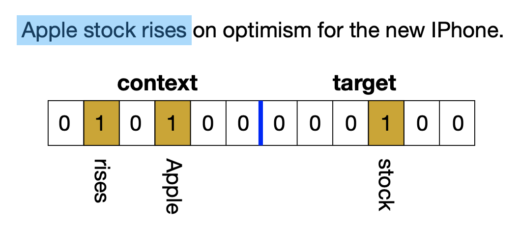Building a bag-of-words representation for each n-gram

Finally, why do I say the author "goes to great lengths" to tell a story? First, as mentioned above, dwelling too much on the biomimetic angle feels forced. Second, when the author compares BioWord to word embedding models like Word2Vec and GloVe, its performance is basically worse than both. Third, as a vector binarization algorithm, BioWord shows no particular advantage over existing methods like RandExp or LSH either. If that were all, it would be fine, but what's even more awkward is that the author also forces a comparison with BERT to highlight its "advantages."

The author first introduces the notion of static/dynamic word embeddings: if the first $V$ dimensions of the bag-of-words vector are all zero, then the resulting $K$-dimensional vector is treated as that word's static embedding; if the first $V$ dimensions depend on the context, then the resulting $K$-dimensional vector is called that word's (BERT-like) dynamic embedding. But honestly, this concept doesn't really hold up. By this logic, even Word2Vec — if you take the average context embedding and concatenate it with the center word's embedding — would count as producing a "dynamic embedding." This is really just something to talk about, and the experimental results don't show any real advantage either. What's more, as a word embedding model, the author even compares training cost against BERT to highlight its own advantage, which is genuinely awkward — and it shows just how hard the author worked to sell this story.

BioHash

BioHash comes from the paper Bio-Inspired Hashing for Unsupervised Similarity Search. It's a method for binarizing vectors, and unlike traditional LSH, it is data-dependent — "custom-tailored" to a specific dataset — so it typically produces sparser, better-performing binary vectors.

Given a set of vectors $\{\boldsymbol{x}_i\}_{i=1}^N$, the BioHash algorithm roughly works as follows:

1. Use K-Means to cluster $\{\boldsymbol{x}_i\}_{i=1}^N$ into $K$ classes, obtaining $K$ cluster centers;
2. Map each $\boldsymbol{x}_i$ to a $K$-dimensional 0/1 vector, where the positions corresponding to the $\boldsymbol{x}_i$ nearest $k$ classes are set to 1, and the rest to 0.

I say "roughly" because there are some discrepancies in the algorithmic details. First, the distance used in the clustering process is not Euclidean distance but a normalized inner product, i.e., $d(\boldsymbol{x}, \boldsymbol{w}) = -\langle \boldsymbol{x}, \boldsymbol{w} / \Vert\boldsymbol{w}\Vert\rangle$ — an approach we've used before when exploring Capsules; readers can refer to Another New Year's Feast: From K-Means to Capsules. Second, when solving for the cluster centers, SGD is used instead of the standard EM algorithm — something I honestly don't quite understand, since although SGD allows mini-batch updates and is friendlier to memory, in principle EM can also be run in batches without necessarily running into memory issues. Finally, the part I find completely baffling is that during clustering, the author uses the normalized inner product $-\langle \boldsymbol{x}, \boldsymbol{w} / \Vert\boldsymbol{w}\Vert\rangle$ as the distance metric, but when deciding which cluster each sample belongs to, switches to the unnormalized inner product $-\langle \boldsymbol{x}, \boldsymbol{w}\rangle$ as the distance instead — which is genuinely puzzling.

That said, setting aside the details of BioHash, its actual performance is quite impressive, so in the right settings, BioHash is well worth borrowing and using. Sharp-eyed readers may notice that BioWord and BioHash share several of the same authors — in fact, they come from the same lab — which makes it easy to understand why BioWord wants to carry forward BioHash's original motivation, just applied to constructing word embeddings instead. In my view, though, whether judged by motivation or by the results reported in the paper, it's hard to call this a particularly elegant piece of work.

FlyHash

Having said all this, we still haven't addressed the question in the title: what exactly does BioWord have to do with fruit flies? Or rather, where in BioHash does the resemblance to fruit flies actually show up? Tracing BioHash's references, we find that BioHash is in fact an improvement on an algorithm called FlyHash — so if we want to trace the origin, we need to look at FlyHash.

As the name suggests, FlyHash is a new vector binarization method conceived mainly by drawing inspiration from the fruit fly's olfactory circuit, and it is more efficient than conventional LSH. For readers unfamiliar with LSH, we'll cover it later in this post; for now, let's go straight into FlyHash. In fact, both FlyHash and LSH follow the idea of "random projection + binarization," except that the fruit fly inspired a new direction for optimization: high dimensionality + low activation.

Specifically, let the original data be $\boldsymbol{x}_i \in \mathbb{R}^{D}$. FlyHash chooses a random binary matrix $\boldsymbol{W}\in\{0,1\}^{D\times K}$ (fixed once chosen), where typically $K > D$ (high-dimensional). After projection, $\boldsymbol{x}_i \boldsymbol{W}$ is a $K$-dimensional vector. A WTA (Winner Take All) operation is then applied to achieve "low activation" — "set the top $k$ largest elements of $\boldsymbol{x}_i \boldsymbol{W}$ to 1, and the rest to 0" — giving us a binary vector with $k$ ones and $K-k$ zeros, which is used as the hash vector for $\boldsymbol{x}_i$.

Since there are only a limited number, $k$, of active elements, even after increasing the dimensionality, the storage and retrieval cost doesn't grow — while performance actually improves. This is precisely the benefit of the "high dimensionality + low activation" idea inspired by the fruit fly. FlyHash was first published in the Science paper A Neural Algorithm for a Fundamental Computing Problem; readers interested in the "high dimensionality + low activation" fruit fly olfactory circuit can consult that paper for details. Later, the paper Improving Similarity Search with High-dimensional Locality-sensitive Hashing further refined the theoretical side; the two papers are very much part of the same lineage.

So now we can answer "how did this end up connected to fruit flies": essentially, any algorithm whose binarization process embodies the "high dimensionality + low activation" idea can be said to be "Inspired by Fly." Since FlyHash relies on random projection to get its final result, it needs to project up to a sufficiently high dimension to guarantee performance, whereas BioHash is trained on the specific dataset at hand, so it typically doesn't need as many dimensions as FlyHash while achieving better performance — but BioHash still clearly embodies the "winner take all" idea, so it too is described as "Inspired by Fly." And since BioWord uses BioHash, it also claims to be "Inspired by Fly."

LSH

Finally, let's briefly introduce LSH (Locality Sensitive Hashing) for readers who aren't familiar with it. A full treatment of LSH could easily fill an entire post on its own, so here we'll focus mainly on the part most closely related to FlyHash.

Simply put, LSH is an algorithm for binarizing vectors such that the binarized vectors approximately preserve the original metric. A common scheme uses random projection to (approximately) preserve cosine similarity. From earlier posts — The Distribution of the Angle Between Two Random Vectors in n-Dimensional Space and Understanding Model Parameter Initialization Strategies from a Geometric Perspective — we know that in high-dimensional space, any two Gaussian random vectors are almost orthogonal. So if we sample $DK$ random numbers from $\mathcal{N}(0,1/n)$ to form a matrix $\boldsymbol{W}\in\mathbb{R}^{D\times K}$, it is "almost" an orthogonal matrix. This means that once two original vectors $\boldsymbol{x}_i, \boldsymbol{x}_j\in\mathbb{R}^{D}$ are each multiplied by $\boldsymbol{W}$, they become two $K$-dimensional vectors whose angle is approximately preserved:

\begin{equation}\cos(\boldsymbol{x}_i \boldsymbol{W}, \boldsymbol{x}_j \boldsymbol{W})\approx \cos(\boldsymbol{x}_i, \boldsymbol{x}_j)\end{equation}

This means that if the retrieval metric is cosine similarity, we can use the projected $\boldsymbol{x} \boldsymbol{W}$ in place of the original vector $\boldsymbol{x}$ for approximate retrieval. Going a step further, after binarizing the result, the cosine similarity is essentially still preserved:

\begin{equation}\boldsymbol{x}\quad\to\quad\text{sgn}(\boldsymbol{x} \boldsymbol{W})\end{equation}

where $\text{sgn}$ is the sign function, converting values greater than 0 to 1 and values less than or equal to 0 to -1, thereby mapping the original vector to a binary vector. Here the target dimension $K$ is generally not larger than $D$, and because the projection is random, we can roughly assume that the result contains about equal numbers of 1s and -1s — which is a clear contrast with FlyHash's "high dimensionality + low activation": whether you treat 1 or -1 as the "active" value, the counts are roughly the same, so this can hardly be called "low activation."

Although the discussion above is only meant as an intuitive guide, there is in fact rigorous probability theory behind it (we've done related theoretical analysis in Performer: Linearizing Attention Complexity via Random Projection as well), so LSH is a rigorous, quantifiable algorithm rather than a purely ad hoc approximation. Once a vector has been binarized, we can treat it as a bag-of-words model (even if the original was a continuous vector), and then build an index on it to accelerate retrieval — an inverted index, for instance. This is the whole point of vector binarization, and vector retrieval libraries such as Faiss all include LSH algorithms.

Summary

This post traced the lineage of a binarized word embedding model, investigating exactly how it ended up connected to fruit flies, and along the way we've also gotten to know the ideas behind — and the relationships among — vector binarization methods such as BioHash, FlyHash, and LSH. This is also the first time I've tried writing in a "reverse chronological" style — hope you enjoyed it~