Performer: Linearizing Attention's Complexity via Random Projections

Performer：用随机投影将Attention的复杂度线性化 苏剑林 · 2020-12-01 · Machine Learning optimization attention

The $\mathcal{O}(n^2)$ complexity of the attention mechanism has long been a thorny issue, and there are mainly two lines of thinking about how to change this complexity: one is the sparsification approach, such as Sparse Attention, which we've covered before, and Google's Big Bird from a few months ago, among others; the other is the linearization approach, which we summarized previously in Exploring Linear Attention: Does Attention Need a Softmax? — readers may want to go back and look at that. This post introduces a new piece of work along the linearization line, Performer, from Google's paper Rethinking Attention with Performers. Its goal is rather bold: through random projections, linearize the complexity of attention without sacrificing accuracy.

Put plainly, in the ideal case we wouldn't need to retrain the model at all, and the output would show no noticeable change, yet the complexity would drop to $\mathcal{O}(n)$! It really does sound like a free lunch falling from the sky — is it really that good? more

Attention

As we know, attention is generally defined as:

\begin{equation}Attention(\boldsymbol{Q},\boldsymbol{K},\boldsymbol{V})_i = \frac{\sum\limits_{j=1}^n \text{sim}(\boldsymbol{q}_i, \boldsymbol{k}_j)\boldsymbol{v}_j}{\sum\limits_{j=1}^n \text{sim}(\boldsymbol{q}_i, \boldsymbol{k}_j)}\label{eq:gen-att}\end{equation}

For standard Scaled-Dot Attention, $\text{sim}(\boldsymbol{q}, \boldsymbol{k})=e^{\boldsymbol{q}\cdot \boldsymbol{k}}$ (sometimes there's also a scaling factor in the exponent, which we won't write explicitly here). Writing the computation over the whole sequence in matrix form gives:

\begin{equation}Attention(\boldsymbol{Q},\boldsymbol{K},\boldsymbol{V}) = softmax\left(\boldsymbol{Q}\boldsymbol{K}^{\top}\right)\boldsymbol{V}\end{equation}

We're mainly concerned with the self-attention setting, so generally $\boldsymbol{Q}, \boldsymbol{K}, \boldsymbol{V}\in\mathbb{R}^{n\times d}$. In the expression above, the step $\boldsymbol{Q}\boldsymbol{K}^{\top}$ amounts to computing inner products between $n^2$ vector pairs, yielding $n^2$ real numbers, so both the time and space complexity are $\mathcal{O}(n^2)$.

For linear attention, on the other hand, $\text{sim}(\boldsymbol{q}, \boldsymbol{k})=\phi(\boldsymbol{q})\cdot \varphi(\boldsymbol{k})$, where $\phi,\varphi$ is an activation function with a non-negative range. In this case, the core computation of attention (the numerator part of equation $\eqref{eq:gen-att}$) becomes

\begin{equation}\left(\phi(\boldsymbol{Q})\varphi(\boldsymbol{K})^{\top}\right)\boldsymbol{V}=\phi(\boldsymbol{Q})\left(\varphi(\boldsymbol{K})^{\top}\boldsymbol{V}\right)\end{equation}

The left-hand side of the equation above still has complexity $\mathcal{O}(n^2)$, but since matrix multiplication is associative, we can compute the product of the latter two matrices first, which brings the complexity down to $\mathcal{O}(n)$. For a detailed explanation, please refer back to the earlier post Exploring Linear Attention: Does Attention Need a Softmax? — we won't expand on it further here.

Performer

Now we can move on to introducing Performer. As mentioned at the outset, Performer's starting point is still standard attention, so it still has $\text{sim}(\boldsymbol{q}, \boldsymbol{k})=e^{\boldsymbol{q}\cdot \boldsymbol{k}}$, and it wants to linearize the complexity, which means finding a new $\tilde{\boldsymbol{q}}, \tilde{\boldsymbol{k}}$ such that:

\begin{equation}\text{sim}(\boldsymbol{q}, \boldsymbol{k}) \approx \tilde{\boldsymbol{q}}\cdot\tilde{\boldsymbol{k}}\end{equation}

Finding a reasonable mapping scheme from $\boldsymbol{q},\boldsymbol{k}$ to $\tilde{\boldsymbol{q}},\tilde{\boldsymbol{k}}$ is precisely the hardest part of this approach.

An elegant random mapping

Performer's greatest contribution is that it found a remarkably elegant mapping scheme:

\begin{equation}\begin{aligned} e^{\boldsymbol{q}\cdot \boldsymbol{k}}&=\mathbb{E}_{\boldsymbol{\omega}\sim \mathcal{N}(\boldsymbol{\omega};0,\boldsymbol{1}_d)}\left[e^{\boldsymbol{\omega}\cdot \boldsymbol{q}-\Vert \boldsymbol{q}\Vert^2 / 2} \times e^{\boldsymbol{\omega}\cdot \boldsymbol{k}-\Vert \boldsymbol{k}\Vert^2 / 2}\right]\\[6pt] &\approx\underbrace{\frac{1}{\sqrt{m}}\begin{pmatrix}e^{\boldsymbol{\omega}_1\cdot \boldsymbol{q}-\Vert \boldsymbol{q}\Vert^2 / 2} \\ e^{\boldsymbol{\omega}_2\cdot \boldsymbol{q}-\Vert \boldsymbol{q}\Vert^2 / 2}\\ \vdots\\ e^{\boldsymbol{\omega}_m\cdot \boldsymbol{q}-\Vert \boldsymbol{q}\Vert^2 / 2} \end{pmatrix}}_{\tilde{\boldsymbol{q}}} \cdot \underbrace{\frac{1}{\sqrt{m}}\begin{pmatrix}e^{\boldsymbol{\omega}_1\cdot \boldsymbol{k}-\Vert \boldsymbol{k}\Vert^2 / 2} \\ e^{\boldsymbol{\omega}_2\cdot \boldsymbol{k}-\Vert \boldsymbol{k}\Vert^2 / 2}\\ \vdots\\ e^{\boldsymbol{\omega}_m\cdot \boldsymbol{k}-\Vert \boldsymbol{k}\Vert^2 / 2} \end{pmatrix}}_{\tilde{\boldsymbol{k}}} \end{aligned}\label{eq:core}\end{equation}

Let's first unpack what this equation is saying. The first equality means the two sides are exactly identical, which implies that if we sample infinitely many $\boldsymbol{\omega}$ from the standard normal distribution $\mathcal{N}(\boldsymbol{\omega};0,\boldsymbol{1}_d)$, and then average $e^{\boldsymbol{\omega}\cdot \boldsymbol{q}-\Vert \boldsymbol{q}\Vert^2 / 2} \times e^{\boldsymbol{\omega}\cdot \boldsymbol{k}-\Vert \boldsymbol{k}\Vert^2 / 2}$, the result equals $e^{\boldsymbol{q}\cdot \boldsymbol{k}}$. Written in integral form:

\begin{equation}\begin{aligned} &\frac{1}{(2\pi)^{d/2}}\int e^{-\Vert\boldsymbol{\omega}\Vert^2 / 2}\times e^{\boldsymbol{\omega}\cdot \boldsymbol{q}-\Vert \boldsymbol{q}\Vert^2 / 2} \times e^{\boldsymbol{\omega}\cdot \boldsymbol{k}-\Vert \boldsymbol{k}\Vert^2 / 2}d\boldsymbol{\omega} \\ =&\frac{1}{(2\pi)^{d/2}}\int e^{-\Vert\boldsymbol{\omega}-\boldsymbol{q}-\boldsymbol{k}\Vert^2 / 2 + \boldsymbol{q}\cdot \boldsymbol{k}}d\boldsymbol{\omega}\\ =&\, e^{\boldsymbol{q}\cdot \boldsymbol{k}} \end{aligned}\end{equation}

Of course, in practice we can only sample a finite number, $m$, of them, which gives us the second, approximate equality. And this can be written exactly as an inner product of two $m$-dimensional vectors — precisely the $e^{\boldsymbol{q}\cdot \boldsymbol{k}}\approx \tilde{\boldsymbol{q}}\cdot\tilde{\boldsymbol{k}}$ we need! So, with this approximation, we can convert the exponential of an inner product of two $d$-dimensional vectors into an inner product of two $m$-dimensional vectors, and thus, in theory, we can convert a standard attention model with head_size $d$ into a linear attention model with head_size $m$. This is the core idea of the entire paper.

A discussion of the derivation

Some readers might be curious about where equation $\eqref{eq:core}$ comes from — let's dig into this a bit; readers who aren't interested can simply skip this section. Although one can verify equation $\eqref{eq:core}$ directly by computing the integral, the question is whether, for an arbitrary $\text{sim}(\boldsymbol{q}, \boldsymbol{k})$, a similar linear approximation can be found. Below we'll show that a similar linearization scheme can indeed be found via a general procedure — though the result may be far less elegant and effective than equation $\eqref{eq:core}$.

Specifically, for an arbitrary $\text{sim}(\boldsymbol{q}, \boldsymbol{k})$, we can rewrite it as

\begin{equation}\text{sim}(\boldsymbol{q}, \boldsymbol{k}) = \frac{\beta(\boldsymbol{q})\gamma(\boldsymbol{k})\text{sim}(\boldsymbol{q}, \boldsymbol{k})}{\beta(\boldsymbol{q})\gamma(\boldsymbol{k})}\end{equation}

and then take the Fourier transform of $\beta(\boldsymbol{q})\gamma(\boldsymbol{k})\text{sim}(\boldsymbol{q}, \boldsymbol{k})$:

\begin{equation}\mathcal{F}(\boldsymbol{\omega}_q, \boldsymbol{\omega}_k)=\frac{1}{(2\pi)^{d/2}}\int \beta(\boldsymbol{q})\gamma(\boldsymbol{k})\text{sim}(\boldsymbol{q}, \boldsymbol{k})e^{-i\boldsymbol{\omega}_q\cdot \boldsymbol{q}-i\boldsymbol{\omega}_k\cdot \boldsymbol{k}}d\boldsymbol{q}d\boldsymbol{k}\end{equation}

As for why we multiply by $\beta(\boldsymbol{q})\gamma(\boldsymbol{k})$ first — this is because taking the Fourier transform of $\text{sim}(\boldsymbol{q}, \boldsymbol{k})$ directly may give an ugly result, or might not even exist, whereas multiplying by a suitable function can fix this. For instance, we can let $\beta(\boldsymbol{x})=\gamma(\boldsymbol{x})=e^{-\lambda\Vert x\Vert^2}$; as long as $\lambda$ is large enough, many $\text{sim}(\boldsymbol{q}, \boldsymbol{k})$ will admit a Fourier transform.

Next we perform the inverse transform and substitute back into the original expression, obtaining

\begin{equation}\text{sim}(\boldsymbol{q}, \boldsymbol{k})=\frac{1}{(2\pi)^{d/2}}\int \mathcal{F}(\boldsymbol{\omega}_q, \boldsymbol{\omega}_k)\frac{e^{i\boldsymbol{\omega}_q\cdot \boldsymbol{q}}}{\beta(\boldsymbol{q})} \frac{e^{i\boldsymbol{\omega}_k\cdot \boldsymbol{k}}}{\gamma(\boldsymbol{k})}d\boldsymbol{\omega}_q d\boldsymbol{\omega}_k\end{equation}

If we can compute $\mathcal{F}(\boldsymbol{\omega}_q, \boldsymbol{\omega}_k)$ and normalize it, it can become a distribution we can sample from, letting us draw a random vector $\boldsymbol{\omega}_q,\boldsymbol{\omega}_k$ and then approximately convert it into the inner product of vectors formed from $\frac{e^{i\boldsymbol{\omega}_q\cdot \boldsymbol{q}}}{\beta(\boldsymbol{q})}, \frac{e^{i\boldsymbol{\omega}_k\cdot \boldsymbol{k}}}{\gamma(\boldsymbol{k})}$. Of course, this computation may involve imaginary numbers, while we generally want to work with real numbers only — but that's not a big problem; we can expand it using Euler's formula $e^{i \theta}=\cos\theta + i\sin\theta$ and keep only the real part throughout, and the overall form won't change much. In principle, this whole procedure can be carried out without much difficulty, but compared with equation $\eqref{eq:core}$, there are two issues: 1) now we need to sample two sets of random variables $\boldsymbol{\omega}_q,\boldsymbol{\omega}_k$, which inflates the variance of the estimate; 2) after keeping only the real part, the result is a combination of $\sin,\cos$ terms, and there's no guarantee that this result is non-negative, so extra clipping is needed.

What's special about equation $\eqref{eq:core}$ is that $e^{\boldsymbol{q}\cdot \boldsymbol{k}}$ can be rewritten as

\begin{equation}e^{\boldsymbol{q}\cdot \boldsymbol{k}} = e^{\Vert \boldsymbol{q}\Vert^2 / 2 + \Vert \boldsymbol{k}\Vert^2 / 2 - \Vert\boldsymbol{q}-\boldsymbol{k}\Vert^2 / 2}\end{equation}

so it only needs to be reduced to a problem in the single variable $\boldsymbol{q}-\boldsymbol{k}$, and the Fourier transform of $e^{-\Vert\boldsymbol{q}-\boldsymbol{k}\Vert^2 / 2}$ happens to be $e^{-\Vert\boldsymbol{\omega}\Vert^2 / 2}$, so taking the inverse transform gives us

\begin{equation}e^{\boldsymbol{q}\cdot \boldsymbol{k}}=\frac{e^{\Vert \boldsymbol{q}\Vert^2 / 2 + \Vert \boldsymbol{k}\Vert^2 / 2}}{(2\pi)^{d/2}}\int e^{-\Vert\boldsymbol{\omega}\Vert^2 / 2 + i \boldsymbol{\omega}\cdot (\boldsymbol{q} - \boldsymbol{k})} d\boldsymbol{\omega}\end{equation}

At this point, if we directly take the real part and expand it, we still get a combination of $\sin,\cos$ terms — this is what the original paper calls the $\text{trig}$-style projection scheme. However, there's an even more clever property that changes everything! Notice that the equation above is an identity, so we can substitute $\boldsymbol{q}\to -i\boldsymbol{q},\boldsymbol{k}\to i\boldsymbol{k}$ on both sides, giving:

\begin{equation}e^{\boldsymbol{q}\cdot \boldsymbol{k}}=\frac{e^{-\Vert \boldsymbol{q}\Vert^2 / 2 - \Vert \boldsymbol{k}\Vert^2 / 2}}{(2\pi)^{d/2}}\int e^{-\Vert\boldsymbol{\omega}\Vert^2 / 2 + \boldsymbol{\omega}\cdot (\boldsymbol{q} + \boldsymbol{k})} d\boldsymbol{\omega}\end{equation}

This is exactly equation $\eqref{eq:core}$. Substituting $\boldsymbol{q}\to -i\boldsymbol{q},\boldsymbol{k}\to i\boldsymbol{k}$ leaves the left-hand side unchanged while completely freeing the right-hand side from imaginary numbers, while also preserving non-negativity — truly a case of many coincidences converging into one, a "one of a kind, no substitute" kind of result.

Reducing variance via orthogonalization

Beyond proposing equation $\eqref{eq:core}$ to linearize standard attention, the original paper also introduces a further enhancement. In equation $\eqref{eq:core}$, the $\boldsymbol{\omega}_1,\boldsymbol{\omega}_2,\cdots,\boldsymbol{\omega}_m$ are drawn independently and identically from $\mathcal{N}(\boldsymbol{\omega};0,\boldsymbol{1}_d)$, and the paper points out that if we orthogonalize the individual $\boldsymbol{\omega}_i$, we can effectively reduce the variance of the estimate and improve the average precision of a single estimation pass.

Note that "orthogonalization" here means keeping the norm of $\boldsymbol{\omega}_i$ unchanged while only performing Gram-Schmidt orthogonalization on its direction. This technique was first proposed, also by Google, in the paper The Unreasonable Effectiveness of Structured Random Orthogonal Embeddings, and the Performer paper devotes a full six pages in its appendix to proving this fact. It obviously wouldn't be appropriate to reproduce those six pages of proof here — so how should we think about why this strategy works?

Actually, the fundamental reason this strategy is effective is the isotropy of the sampling distribution $\mathcal{N}(\boldsymbol{\omega};0,\boldsymbol{1}_d)$: its probability density function $(2\pi)^{-d/2}e^{-\Vert\boldsymbol{\omega}\Vert^2 / 2}$ depends only on the norm $\Vert\boldsymbol{\omega}\Vert$ of $\boldsymbol{\omega}$, so it's uniform in direction. If we want to reduce the variance of the estimate, we should reduce the randomness of the sampling, making the sampled results more uniform. Orthogonalizing the individual vectors is one way to achieve directional uniformity — in other words, orthogonalizing the $\boldsymbol{\omega}_i$ promotes uniformity in the sampled results, thereby reducing the variance of the estimate. In addition, the orthogonalization operation is generally only valid for $m\leq d$; if $m > d$, the original paper's approach is to orthogonalize in groups of $d$ vectors at a time.

By analogy, we can see that orthogonalization only makes the sampled directions more uniform; if we want to go even further, we could also make the sampled norms more uniform. Specifically, transforming the standard normal distribution into $d$-dimensional spherical coordinates, the probability element becomes:

\begin{equation}\frac{1}{(2\pi)^{d/2}} r^{d-1} e^{-r^2 /2} dr dS\end{equation}

where $dS = \sin^{d-2}\varphi_{1} \sin^{d-3}\varphi_{2} \cdots \sin\varphi_{d-2}\,d\varphi_{1}\,d\varphi_{2}\cdots d\varphi_{d-1}$ represents the integration element on the $d$-dimensional sphere. This shows that the standard normal distribution is uniform in direction, while the probability density of the norm is proportional to $r^{d-1} e^{-r^2 /2}$. Let's define its cumulative distribution function:

\begin{equation}P_d(r\leq R) = \frac{\int_0^R r^{d-1} e^{-r^2 /2} dr}{\int_0^{\infty} r^{d-1} e^{-r^2 /2} dr}\end{equation}

If we want to sample $m$ samples, we can set $P_d(r\leq R_i) = \frac{i}{m+1},\,i=1,2,\cdots,m$ and solve for $m$ values of $R_i$ to use as norms.

Performance and results

That covers the theory — and it's already gone on a fair bit longer than usual. Generally speaking, if you already have some understanding of linear attention, once you see equation $\eqref{eq:core}$ you'll quickly grasp the essence of Performer; everything else is icing on the cake and doesn't affect the main thread of the story. Next let's look at the evaluation of Performer.

Evaluation in the original paper

Let's first look at the evaluation in the original paper. It is actually quite extensive, but a bit disorganized, and for readers mainly interested in NLP it might feel somewhat puzzling in places.

First up is the speed comparison — unsurprisingly, once the sequence gets long, Performer shows a clear advantage over standard Transformers:

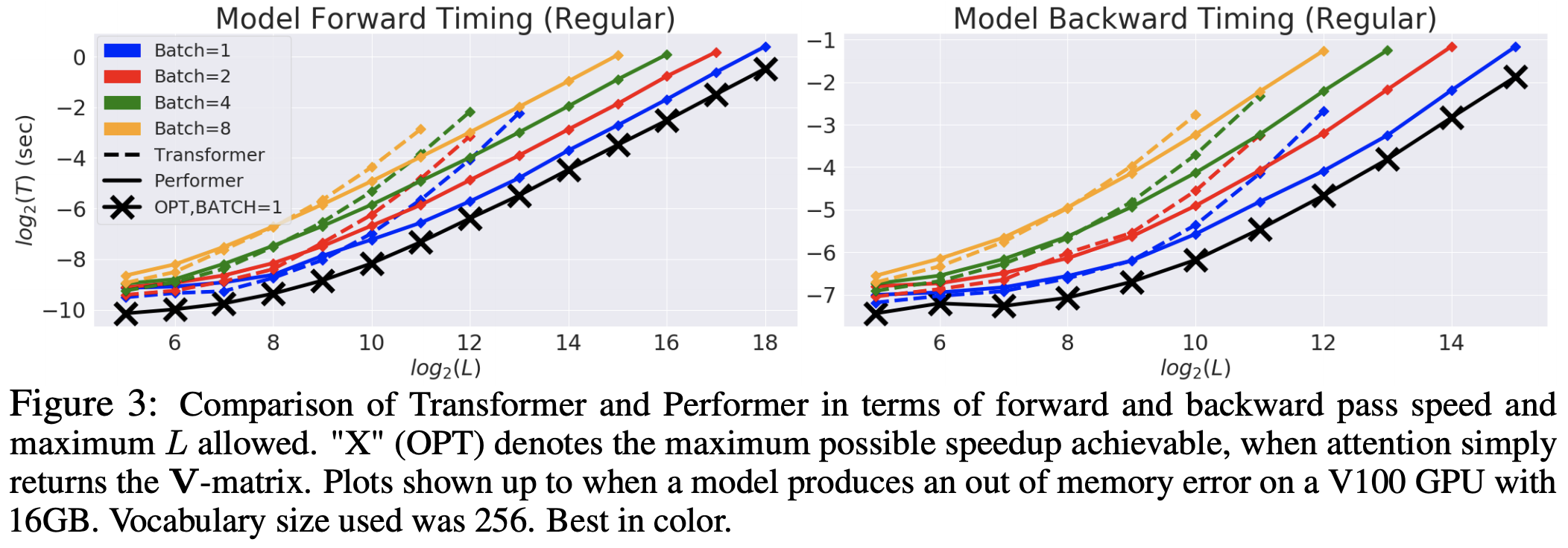Speed comparison between Performer and standard Transformer (solid line: Performer, dashed line: standard Transformer)

Next is a comparison of approximation quality, demonstrating the effectiveness of orthogonalizing the sampled vectors, and the accuracy of the proposed equation $\eqref{eq:core}$ relative to the older $\sin,\cos$-function-based form:

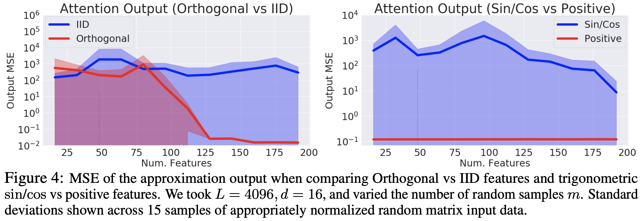Left: comparing the effectiveness of orthogonalizing the sampled vectors; Right: comparing the accuracy of Performer's approximation against the older trigonometric-function-based approximation

So, can it achieve our original hoped-for goal — using an already-trained model's weights without retraining? Unfortunately, no. The original paper ran two experiments showing that loading a standard Transformer's weights directly into Performer fails to reproduce the existing results, though after fine-tuning it can quickly recover them. The paper doesn't offer much analysis as to why this fails to reproduce well initially.

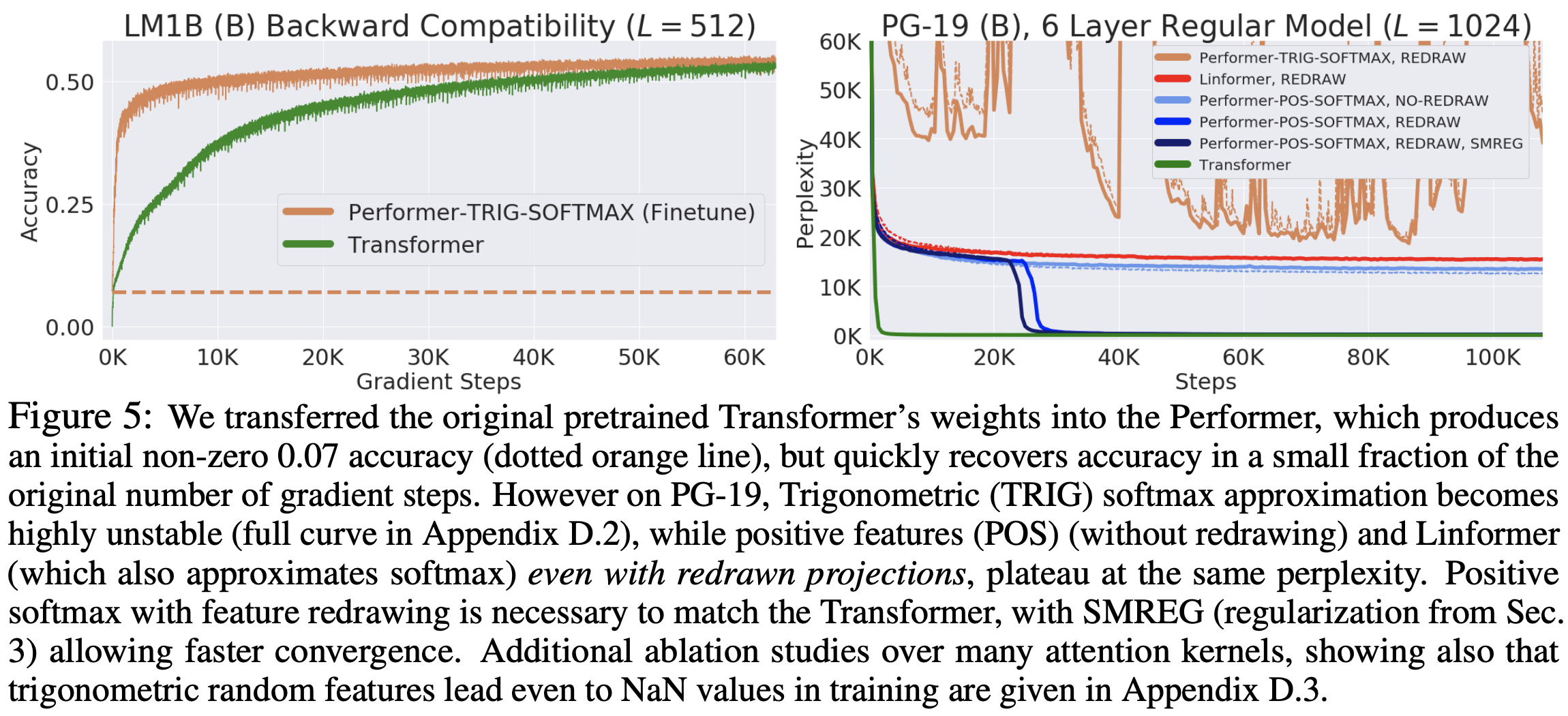Experiment loading Performer with pretrained Transformer weights

Finally, the paper also runs experiments on protein sequences and images, showing that Performer is effective for long sequences — in particular, at least more effective than Reformer. That's roughly the extent of the experiments in the paper: there's a lot of content, but it can feel a bit unfocused.

Evaluations from other papers

Perhaps even Google's own colleagues found this a bit much, because later Google put out two more papers, Efficient Transformers: A Survey and Long Range Arena: A Benchmark for Efficient Transformers, which systematically evaluate and compare various existing methods for improving Transformer efficiency, including Performer. By comparison, the results presented in these two papers are much more intuitive — a few simple charts make clear where each model stands.

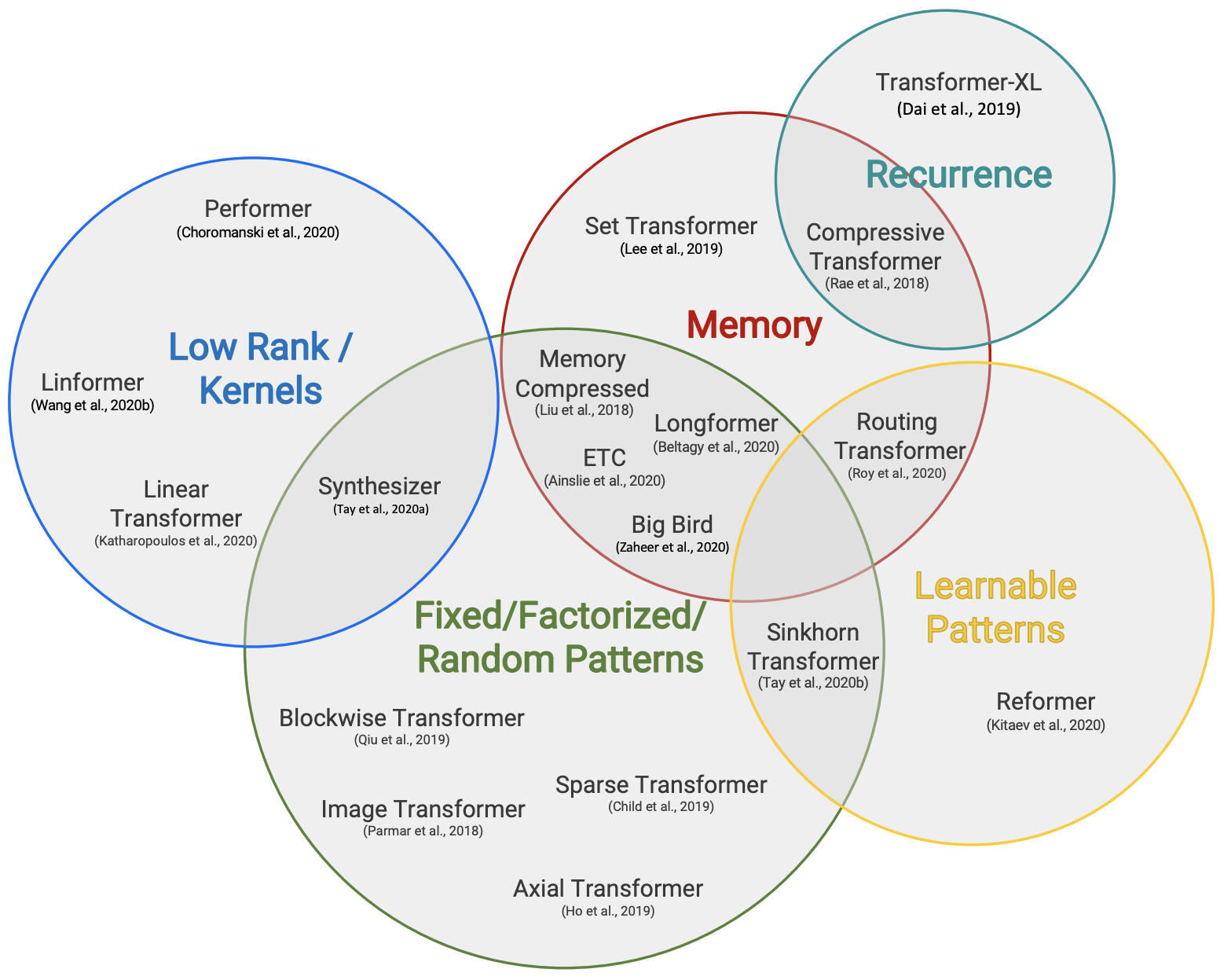Categorization of various efficient Transformers

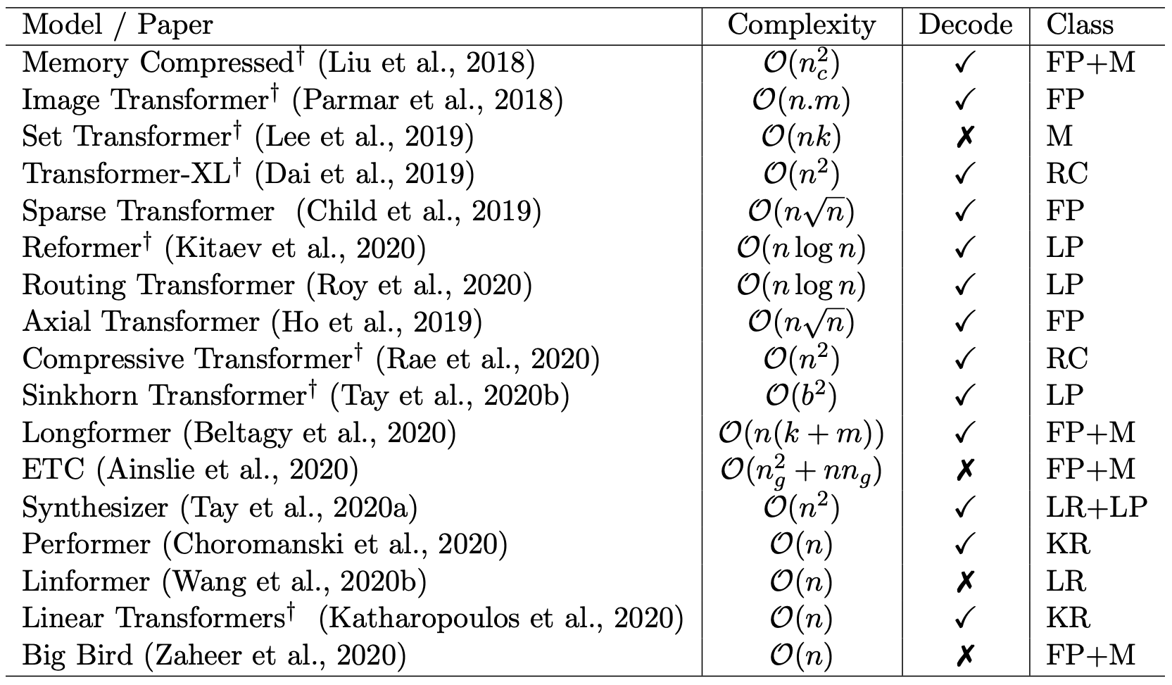Comparison of various improved Transformer variants. The "decode" column indicates whether the model can mask out future information, for use as a language model

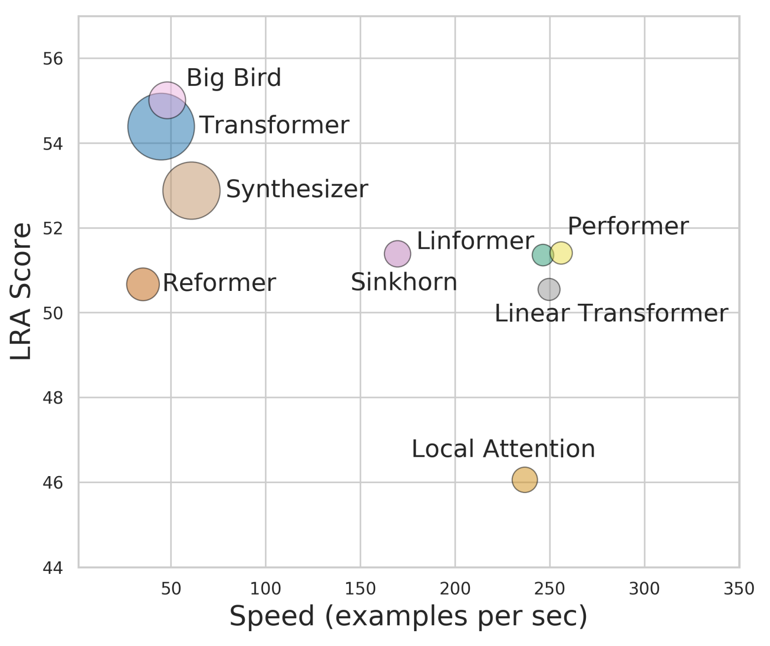"Performance-speed-memory" chart for each Transformer model, where the vertical axis is performance, the horizontal axis is speed, and the circle size represents the GPU memory required. In theory, the closer to the upper right and the smaller the circle, the better the model

For more detailed evaluation information, readers are encouraged to check out these two papers themselves.

Issues and reflections

Performer sounds pretty good so far — does that mean we should just replace Transformer with it? Not quite. Despite its many merits, Performer still has some unresolved issues.

First, in order to better approximate standard Transformer, Performer's $m$ needs to be set fairly large — at least $m > d$, generally several times $d$. This means Performer's head_size needs to be noticeably larger than that of a standard Transformer. Although in theory, no matter how large $m$ is, as long as it's fixed, Performer's complexity is linear in sequence length, when $m$ gets larger, the amount of computation increases noticeably for shorter sequences. In other words, for short sequences, Performer's performance should actually degrade. Based on the author's estimate, only when the sequence length exceeds about 5000 does Performer show a clear advantage.

Second, as things stand, Performer (like other linear attention methods) is incompatible with relative position encoding, since relative position encoding is added directly into the attention matrix — and Performer doesn't even have an explicit attention matrix, so there's nowhere to add it. Furthermore, special seq2seq setups like UniLM also become impossible, though ordinary unidirectional language modeling is still fine. In short, the explicit $\mathcal{O}(n^2)$ attention matrix actually brings a great deal of flexibility, and linear attention, by abandoning that attention matrix, also gives up this flexibility.

Finally — and this is, in the author's view, the biggest issue — Performer's whole idea is to linearize standard attention, so why not just directly train a linear attention model from the start, rather than trying to approximate standard attention? Looking at the last chart above, Performer doesn't show a clear advantage over the Linear Transformer (and in fact, the author suspects there might be something off about that comparison in the last chart: Performer might indeed perform somewhat better than Linear Transformer, but how could it possibly be faster too? Performer itself is converted into a form of linear attention, with an extra conversion step on top — how could it end up faster?). So the value of Performer remains something of an open question, especially since implementing linear attention directly is much simpler, and it works uniformly well for both long and short sequences, whereas implementing Performer is considerably more involved and only pays off for long sequences.

Summary

This post mainly introduced Google's new model Performer, a piece of work that linearizes the complexity of standard attention through random projections. There's plenty in it worth learning from. Finally, we summarized the evaluation results of various improved Transformer variants, and shared the author's own reflections on Performer.