Another New Year Feast: From K-Means to Capsule

再来一顿贺岁宴：从K-Means到Capsule 苏剑林 · 2018-02-12 · Machine Learning deep learning clustering capsule

In this post, I'll take yet another pass at analyzing Capsule.

Overall, the details of the Capsule algorithm are not that complicated—implementing Capsule with a framework by following its procedure should present no problems. The hard part is understanding what Capsule is actually doing, and why it's designed this way, especially those Dynamic Routing steps.

Why do I keep coming back to analyze Capsule? This isn't simply "reheating leftovers," but rather an attempt to arrive at a genuine understanding of Capsule's underlying principles. As everyone knows, Capsule tends to leave people with the impression of being "full of arbitrary human conventions," lacking that intuitive sense of "even though I don't fully get it, I believe it must be this way." I want to think through Capsule's whole story as thoroughly as possible, so that we can come to see it as a natural, coherent model—one we might even be able to generalize from.

In Lifting the Fog: A Delicious Feast of Capsules, I first analyzed the results of dynamic routing, and then argued that the output is some kind of clustering of the input—this "from result to cause" process involved a fair amount of guesswork based on surface appearances. This time, I'll go the other way: I'll start by confirming directly that the output is a clustering of the input, and then work backward to derive what dynamic routing should look like, which involves much less hand-waving. The two posts complement each other to some extent. more

The Capsule Framework

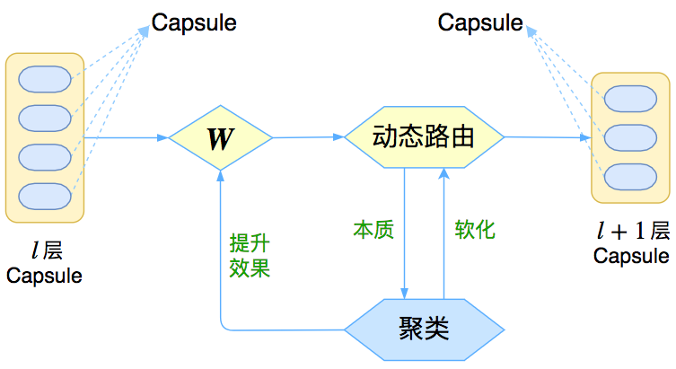Figure 1: A concise schematic of the Capsule framework

Rather than calling Capsule a specific model, it's better described as a modeling framework, where the content of each step within the framework can be freely swapped out. The paper Hinton published is just one particular use case.

So what kind of framework is this?

Feature Representation

In the Capsule model, every feature is represented by a vector (i.e., a capsule).

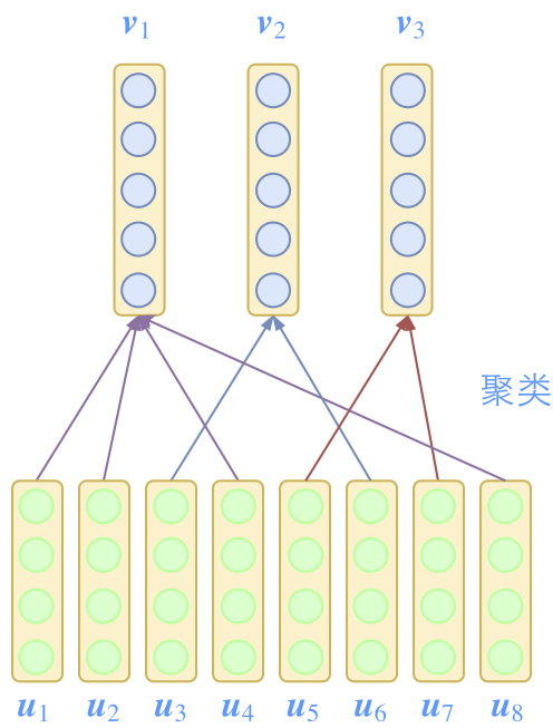Figure 2: Every feature in Capsule is a vector, and features progress upward through clustering

Of course, for readers who follow the news, this is nothing new. Some readers might wonder: what's so special about representing features as vectors—isn't the feature input to a neural network already a vector? Well, originally, the input to each layer of an MLP is a vector $\boldsymbol{x}\in\mathbb{R}^n$, and the output is $\boldsymbol{y}=Activation(\boldsymbol{W}\boldsymbol{x}+\boldsymbol{b})\in \mathbb{R}^k$; we'd treat each component of $\boldsymbol{x}$ as a feature, so each feature is a scalar. Once features are "vectorized," the input to each layer becomes $\boldsymbol{x}\in\mathbb{R}^{n\times d_x}$, and the output becomes $\boldsymbol{y}=Routing(\boldsymbol{x})\in \mathbb{R}^{k\times d_y}$. Now the input $\boldsymbol{x}$ is regarded as $n$ features, but each feature is a $d_x$-dimensional vector; the output $\boldsymbol{y}$ is regarded as $k$ features, each an $d_y$-dimensional vector. Put another way, the input and output of each MLP layer go from being a single vector to being a collection of vectors (a matrix).

We could also give this a different name: "distributed representation of features." Readers who spot the phrase "distributed representation" might think of word embeddings in NLP. Indeed, word embeddings were originally called "Distributed Representation," and when I first noticed this property of Capsule, my first reaction was exactly this analogy with word embeddings. We can use word embeddings instead of one-hot encodings to represent a word, which conveys much richer information, and moreover all words live in the same vector space, making downstream processing easier.

Beyond that, there's actually a precedent in images: as everyone knows, a color image typically has three channels, R, G, B, each with 256 choices, giving $256^3=16777216$ possible colors in total (roughly 17 million). Why not just use 17 million distinct numbers to represent these colors directly, instead of splitting them into 3 groups of 256 numbers each? This too is a form of distributed representation, and it lets us better express the diversity of colors (for instance, what color is "close to" red? Some might say orange, others purple, still others pink—a single number can't capture multiple kinds of similarity at once, but a grouped representation can). Going further, whenever we repeatedly apply convolution to an image, the resulting channel dimension is itself a kind of distributed representation of image features.

Feature Combination

The second characteristic of Capsule is that features are combined via clustering.

Combination and Representation

Combining lower-level features into higher-level ones is consistent with how our own cognition works. In NLP, we have the progression "character → word → sentence → paragraph"; in vision, we have "point → line → surface → volume." When faced with something new (a higher-level feature), we always decompose it into things we're already familiar with (lower-level features), and then mentally map those familiar things onto this new thing (feature combination).

For us, this process of decomposition and combination doesn't necessarily serve any particular purpose—it's simply how we make sense of new things in our own way (forming a good feature representation in the brain). This also helps explain one of the reasons Hinton criticizes deep learning and has been pushing Capsule instead: he feels that current deep learning models are too task-specific (for example, an MNIST classification model can only recognize a single digit; recognizing multiple digits would require building a new dataset and redesigning and retraining the model from scratch). In reality, our fundamental goal isn't simply to perform tasks, but to use tasks as a vehicle for forming good, general-purpose feature representations—only this way can we hope to arrive at genuine artificial intelligence.

Clustering Between Features

So how is this combination process actually carried out? Consider: why do two characters become a word? Because these two characters frequently appear "clustered together," and moreover this "cluster" consists only of the two of them. This tells us that features aggregate because they exhibit a tendency to cluster, and so Capsule builds a clustering algorithm right into the model.

Note that the clustering we've discussed before was always clustering between samples—for instance, automatically clustering MNIST images into 10 categories, or clustering word vectors trained via Word2Vec into several groups, where the object being clustered is a sample (an input). Capsule, by contrast, represents the input itself as several feature vectors, and then clusters these vectors (clustering between features) to obtain several center vectors; it then clusters those center vectors again, progressing layer by layer to complete a process of successive abstraction. This is clustering between features.

Now the question arises: given that it's clustering, what method is used to do the clustering? And then, how do we derive that mysterious Dynamic Routing procedure from this clustering method? Later on we'll trace things back to K-Means to get to the bottom of it, but for now let's finish laying out the main line of thought.

Feature Salience

Combining features gives us higher-level features, but how do we compare the strength of different features? Capsule's answer: vector norm. It's like trying to spot the "standout" among a sea of vectors—you just look at who's "taller." So using the norm of a feature vector to measure its own degree of "prominence" is a fairly natural choice. In addition, we'd like this measure to be bounded, so we apply a squashing operation to the feature vector:

$$squash(\boldsymbol{v})=\frac{\Vert\boldsymbol{v}\Vert^2}{1+\Vert\boldsymbol{v}\Vert^2}\frac{\boldsymbol{v}}{\Vert\boldsymbol{v}\Vert}\tag{1}$$

The squashing scheme isn't unique, and I won't go into it further here. That said, in my experiments I found that replacing the 1 with 0.5 improves performance.

Figure 3: Capsule characterizes the combined nature of features via clustering of feature vectors

To bring out this meaning of the norm, the model design needs to cooperate accordingly. As shown in the figure, although the feature vectors $\boldsymbol{u}_1,\boldsymbol{u}_2,\boldsymbol{u}_4,\boldsymbol{u}_8$ belonging to the class represented by $\boldsymbol{v}_1$ each individually have small norms, because there are many members ("many followers"), the norm of $\boldsymbol{v}_1$ can still come out on top ("strength in numbers"). This shows that how prominent a class is depends both on the number of vectors in that class and on the norms of the individual vectors within it. Later we'll see how Capsule embodies this idea.

Revisiting K-Means

Since this post keeps emphasizing that Capsule abstracts features through clustering, it's worth taking a closer look at clustering algorithms. The clustering algorithm used by Capsule is actually a variant of K-Means. There are many clustering algorithms, and in principle any of them could work, but embedding a clustering algorithm into Capsule does require a bit of care.

The Clustering Objective

K-Means clustering is essentially a "center-based clustering method"—clustering means finding class centers. To define a center, we need a measure of closeness; the Euclidean distance is commonly used, but it's not the only option. So let's introduce K-Means within a more general framework: K-Means aims to partition existing data $\boldsymbol{u}_1, \boldsymbol{u}_2, \dots, \boldsymbol{u}_n$ into $k$ classes in an unsupervised manner, by finding $k$ cluster centers $\boldsymbol{v}_1, \boldsymbol{v}_2, \dots, \boldsymbol{v}_k$ that minimize the within-class spread:

$$L=\sum_{i=1}^n \min_{j=1}^k d(\boldsymbol{u}_i, \boldsymbol{v}_j)\tag{2}$$

Here $d$ represents the measure of closeness, so the idea of this expression is simple: each $\boldsymbol{u}_i$ belongs only to the class it's closest to, and then we sum up all the within-class distances and minimize this total within-class distance:

$$(\boldsymbol{v}_1, \dots, \boldsymbol{v}_k) = \mathop{\text{argmin}}_{(\boldsymbol{v}_1, \dots, \boldsymbol{v}_k)}L\tag{3}$$

Note: Clearly, the clustering result depends on the specific form of $d$, which tells us something important: the difference between unsupervised and supervised learning lies in how we "communicate" with the model. In supervised learning, we convey our intent to the model through labeled data; in unsupervised learning, we accomplish this by designing an appropriate metric $d$.

The Solution Process

How do we minimize $L$ to find each center? If you'd rather skip the derivation, feel free to jump to the next section.

Since $L$ contains the operation $\min$, computing its gradient directly is problematic (not impossible, but troublesome near critical points)—in fact, many similar problems remain poorly solved precisely because their loss contains $\min$ (we'll discuss this issue on some other occasion).

However, here we can "soften" this $L$ so that it becomes differentiable. We have a rather elegant formula for this (see In Search of a Smooth Maximum Function):

$$\begin{aligned}\max(\lambda_1,\lambda_2,\dots,\lambda_n)=&\lim_{K\to+\infty}\frac{1}{K}\ln\left(\sum_{i=1}^n e^{\lambda_i K}\right)\\ \approx&\frac{1}{K}\ln\left(\sum_{i=1}^n e^{\lambda_i K}\right)\end{aligned}\tag{4}$$

Note: if we take $K=1$, then clearly the term inside the brackets is exactly the denominator of softmax—which is where the name "softmax" comes from: "soft" plus "max," a "soft maximum."

And we also have

$$\min(\lambda_1,\lambda_2,\dots,\lambda_n)=-\max(-\lambda_1,-\lambda_2,\dots,-\lambda_n)\tag{5}$$

Therefore we obtain

$$L\approx-\frac{1}{K}\sum_{i=1}^n \ln\left(\sum_{j=1}^k e^{-K\cdot d(\boldsymbol{u}_i, \boldsymbol{v}_j)}\right)=-\frac{1}{K}\sum_{i=1}^n\ln Z_i\tag{6}$$

This approximate loss is now smooth and differentiable everywhere, so we can go ahead and compute its gradient:

$$\frac{\partial L}{\partial \boldsymbol{v}_j}\approx\sum_{i=1}^n \frac{e^{-K\cdot d(\boldsymbol{u}_i, \boldsymbol{v}_j)}}{Z_i} \frac{\partial d(\boldsymbol{u}_i, \boldsymbol{v}_j)}{\partial \boldsymbol{v}_j}=\sum_{i=1}^n c_{ij}\frac{\partial d(\boldsymbol{u}_i, \boldsymbol{v}_j)}{\partial \boldsymbol{v}_j}\tag{7}$$

Here

$$c_{ij}=\mathop{softmax}\limits_j\Big(-K\cdot d(\boldsymbol{u}_i, \boldsymbol{v}_j)\Big)$$

we've explicitly indicated normalization along the dimension indexed by $j$. To find a minimum, we'd like to set $\partial L/\partial \boldsymbol{v}_j=0$, but the resulting equation isn't simple to solve directly. So instead we introduce an iterative process: suppose $\boldsymbol{v}^{(r)}_j$ is the result of the $r$-th iteration of $\boldsymbol{v}_j$; then we can let

$$0=\sum_{i=1}^n c_{ij}^{(r)}\frac{\partial d(\boldsymbol{u}_i, \boldsymbol{v}_j^{(r+1)})}{\partial \boldsymbol{v}_j^{(r+1)}}\tag{8}$$

If we can solve for $\boldsymbol{v}_j^{(r+1)}$ from the equation above, we obtain an iterative scheme.

Euclidean Distance

Now we can substitute our chosen metric into expression $(8)$ and compute. Let's look at the most basic example: $d(\boldsymbol{u}_i, \boldsymbol{v}_j)=\Vert\boldsymbol{u}_i - \boldsymbol{v}_j\Vert^2$, in which case we have

$$\frac{\partial d(\boldsymbol{u}_i, \boldsymbol{v}_j)}{\partial \boldsymbol{v}_j}=2(\boldsymbol{v}_j-\boldsymbol{u}_i)\tag{9}$$

From expression $(8)$ we get $0=2\sum\limits_{i=1}^n c_{ij}^{(r)}\left(\boldsymbol{v}_j^{(r+1)}-\boldsymbol{u}_i\right)$, from which we can solve

$$v_{j}^{(r+1)}=\frac{\sum\limits_{i=1}^n c_{ij}^{(r)}\boldsymbol{u}_i}{\sum\limits_{i=1}^n c_{ij}^{(r)}}\tag{10}$$

If we take the limit $K\to+\infty$, then $c_{ij}^{(r)}$ becomes either 0 or 1, so the above expression says (readers can fill in the proof themselves):

$\boldsymbol{v}_{j}^{(r+1)}$ is the average of those $\boldsymbol{u}_i$ closest to $\boldsymbol{v}_{j}^{(r)}$.

This gives us exactly the ordinary K-Means clustering algorithm we're all familiar with.

Inner-Product Similarity

Euclidean distance isn't well suited to Capsule, because the center vector obtained under Euclidean distance is simply the average of the vectors in the class—meaning that having more vectors in a class doesn't cause the norm of the center vector to grow, which fails to satisfy our earlier design principle that "more followers means more strength."

So what kind of distance would be suitable? The paper "Dynamic Routing Between Capsules" states:

The initial coupling coefficients are then iteratively refined by measuring the agreement between the current output $\boldsymbol{v}_j$ of each capsule, $j$, in the layer above and the prediction $\boldsymbol{\hat{u}_{j|i}}$ made by capsule $i$.
The agreement is simply the scalar product $a_{ij} = \boldsymbol{v}_j \cdot \boldsymbol{\hat{u}_{j|i}}$ ...

Translated into our terms, the rough idea is to use the inner product $\langle\boldsymbol{u}_i, \boldsymbol{v}_j\rangle$ as the similarity measure, i.e., $d(\boldsymbol{u}_i, \boldsymbol{v}_j)=-\langle\boldsymbol{u}_i, \boldsymbol{v}_j\rangle$. But thinking it through carefully reveals a problem: such a $d$ is unbounded below! A function unbounded below cannot serve as a loss, so this puzzled me for quite a while. Until one day it occurred to me that we could first normalize $\boldsymbol{v}_j$ and then compute the inner product, which effectively gives us:

$$d(\boldsymbol{u}_i, \boldsymbol{v}_j)=-\left\langle\boldsymbol{u}_i, \frac{\boldsymbol{v}_j}{\Vert\boldsymbol{v}_j\Vert}\right\rangle\tag{11}$$

Now, for a fixed $\boldsymbol{u}_i$, no matter how $\boldsymbol{v}_j$ varies, $d(\boldsymbol{u}_i, \boldsymbol{v}_j)$ is bounded below. So this $d$ can indeed serve as a loss. Substituting it into expression $(8)$ and computing, we ultimately obtain

$$\frac{\boldsymbol{v}_j^{(r+1)}}{\left\Vert\boldsymbol{v}_j^{(r+1)}\right\Vert}=\frac{\sum\limits_{i=1}^n c_{ij}^{(r)}\boldsymbol{u}_i}{\left\Vert\sum\limits_{i=1}^n c_{ij}^{(r)}\boldsymbol{u}_i\right\Vert}\tag{12}$$

This says that $\boldsymbol{v}_j^{(r+1)}$ and $\sum\limits_{i=1}^n c_{ij}^{(r)}\boldsymbol{u}_i$ point in the same direction, though this doesn't mean they're equal. Still, this does mean we're free to simply take

$$\boldsymbol{v}_j^{(r+1)}=\sum\limits_{i=1}^n c_{ij}^{(r)}\boldsymbol{u}_i\tag{13}$$

If we take the limit $K\to +\infty$, this becomes:

$\boldsymbol{v}_{j}^{(r+1)}$ is the sum of those $\boldsymbol{u}_i$ closest to $\boldsymbol{v}_{j}^{(r)}$.

Since we're now summing rather than averaging, we finally capture the "more followers, more strength" property. (Note that although both the Euclidean and inner-product cases involve the word "closest," the meaning of "closest" differs between the two, since the metric $d$ used is different.)

Note: derivation of expression $(12)$.
$$\begin{aligned}\frac{\partial\left\langle\boldsymbol{u}_i, \frac{\boldsymbol{v}_j}{\Vert\boldsymbol{v}_j\Vert}\right\rangle}{\partial \boldsymbol{v}_j}=&\frac{\partial \left(\boldsymbol{u}_i \cdot \frac{\boldsymbol{v}_j}{\Vert\boldsymbol{v}_j\Vert}\right)}{\partial \boldsymbol{v}_j}\\ > =&\frac{\boldsymbol{u}_i}{\Vert\boldsymbol{v}_j\Vert}+(\boldsymbol{u}_i \cdot \boldsymbol{v}_j)\frac{\partial}{\partial \boldsymbol{v}_j}\frac{1}{\Vert\boldsymbol{v}_j\Vert}\\ > =&\frac{\boldsymbol{u}_i}{\Vert\boldsymbol{v}_j\Vert}-(\boldsymbol{u}_i \cdot \boldsymbol{v}_j)\frac{\boldsymbol{v}_j}{\Vert\boldsymbol{v}_j\Vert^3}\end{aligned}$$
Then, by expression $(8)$, we get
$$0=\frac{\sum\limits_{i=1}^n C_{ij}^{(r)}\boldsymbol{u}_i}{\left\Vert\boldsymbol{v}_j^{(r+1)}\right\Vert}-\left(\sum\limits_{i=1}^n C_{ij}^{(r)}\boldsymbol{u}_i \cdot \boldsymbol{v}_j^{(r+1)}\right)\frac{\boldsymbol{v}_j^{(r+1)}}{\left\Vert\boldsymbol{v}_j^{(r+1)}\right\Vert^3}$$
Rearranging gives
$$\sum\limits_{i=1}^n C_{ij}^{(r)}\boldsymbol{u}_i=\left(\sum\limits_{i=1}^n C_{ij}^{(r)}\boldsymbol{u}_i \cdot \frac{\boldsymbol{v}_j^{(r+1)}}{\left\Vert\boldsymbol{v}_j^{(r+1)}\right\Vert}\right)\frac{\boldsymbol{v}_j^{(r+1)}}{\left\Vert\boldsymbol{v}_j^{(r+1)}\right\Vert}$$
Taking norms on both sides:
$$\left\Vert\sum\limits_{i=1}^n C_{ij}^{(r)}\boldsymbol{u}_i\right\Vert=\left|\sum\limits_{i=1}^n C_{ij}^{(r)}\boldsymbol{u}_i \cdot \frac{\boldsymbol{v}_j^{(r+1)}}{\left\Vert\boldsymbol{v}_j^{(r+1)}\right\Vert}\right|=\left\Vert\sum\limits_{i=1}^n C_{ij}^{(r)}\boldsymbol{u}_i\right\Vert \times |\cos\theta|$$
Here $\theta$ is the angle between vector $\sum\limits_{i=1}^n C_{ij}^{(r)}\boldsymbol{u}_i$ and vector $\boldsymbol{v}_j^{(r+1)}$, and the above expression shows that $|\cos\theta|=1$, so either $\theta=0$ or $\pi$; $\theta=\pi$ is in fact a maximum rather than a minimum, so $\theta=0$, i.e., they point in the same direction, which gives us expression $(12)$.

Dynamic Routing

After this long preparation, the Dynamic Routing algorithm is finally about to emerge.

As discussed in the first part, each layer of Capsule combines and abstracts features through clustering between features, and clustering requires repeated iteration—it's an implicit process. What we need is a smooth, explicit expression for each layer, $$\boldsymbol{v}_j=\boldsymbol{f}_j(\boldsymbol{u}_1,\dots,\boldsymbol{u}_n)\tag{14}$$
in order to actually train the model. Dynamic routing is precisely the process of using iteration to write down this (approximate) explicit expression.

Basic Steps

Suppose Capsule's input features are $\boldsymbol{u}_1, \boldsymbol{u}_2, \dots, \boldsymbol{u}_n$, and the feature vector of the next layer is $\boldsymbol{v}_1,\boldsymbol{v}_2,\dots,\boldsymbol{v}_k$, which is the cluster center obtained by grouping the previous layer's $n$ vectors into $k$ classes, using the normalized inner product as the clustering measure. Then we can write down the iterative process:

Initialize $\boldsymbol{v}_{j} \leftarrow \boldsymbol{v}_{j}^{(0)}$
Iterate $r$ times:
$\boldsymbol{v}_{j} \leftarrow \boldsymbol{v}_{j}/\Vert\boldsymbol{v}_{j}\Vert$;
if $j=\mathop{\text{argmax}}\limits_{j=1,\dots,k}\langle\boldsymbol{u}_i,\boldsymbol{v}_j\rangle$, then $c_{ij} \leftarrow 1$, otherwise $c_{ij} \leftarrow 0$;
$\boldsymbol{v}_{j} \leftarrow \sum\limits_{i}c_{ij}\boldsymbol{u}_{i}$;
Return $squash(\boldsymbol{v}_j)$.

This version is easy to understand, but because of the operation $\text{argmax}$, we cannot use gradient descent, which is currently the only way to learn the model's other parameters. To work around this, instead of taking the limit $K\to+\infty$, we use a constant $K > 0$, giving:

Initialize $\boldsymbol{v}_{j} \leftarrow \boldsymbol{v}_{j}^{(0)}$
Iterate $r$ times:
$\boldsymbol{v}_{j} \leftarrow \boldsymbol{v}_{j}/\Vert\boldsymbol{v}_{j}\Vert$;
$c_{ij} \leftarrow \mathop{softmax}\limits_j \Big(\langle\boldsymbol{u}_i,K\boldsymbol{v}_j\rangle\Big)$;
$\boldsymbol{v}_{j} \leftarrow \sum\limits_{i}c_{ij}\boldsymbol{u}_{i}$;
Return $squash(\boldsymbol{v}_j)$.

But this introduces a new parameter, $K$: intuitively, too large an $K$ causes vanishing gradients, while too small an $K$ isn't accurate enough, and it's hard to pin down. As we'll see later, though, we can simply set $K=1$ directly, because the solution space for $K=1$ already contains the solutions for any $K$. In the end we arrive at:

Initialize $\boldsymbol{v}_{j}=\boldsymbol{v}_{j}^{(0)}$
Iterate $r$ times:
$\boldsymbol{v}_{j} \leftarrow \boldsymbol{v}_{j}/\Vert\boldsymbol{v}_{j}\Vert$;
$c_{ij} \leftarrow \mathop{softmax}\limits_j \Big(\langle\boldsymbol{u}_i, \boldsymbol{v}_j\rangle\Big)$;
$\boldsymbol{v}_{j} \leftarrow \sum\limits_{i}c_{ij}\boldsymbol{u}_{i}$;
Return $squash(\boldsymbol{v}_j)$.

Interestingly, the result derived this way differs both from Hinton's original paper "Dynamic Routing Between Capsules" and from my earlier introduction. The most notable difference is that $squash(\boldsymbol{v}_j)$ has been replaced by $\boldsymbol{v}_{j}/\Vert\boldsymbol{v}_{j}\Vert$ during the iterations, and squashing is applied only at the very final output. Experiments show this improves the model's feature expressiveness: in the digit experiments from my earlier post (training on single digits, predicting on double digits), it achieves over 95% accuracy (up from the original 91%).

Three Symptoms

Are we done now? Far from it. There are still several issues to address.

1. How do we properly initialize the classes? Since the clustering outcome depends on the initialization, and a good initialization is often half the battle in successful clustering. Now that we're embedding this clustering process into the model as one of its components, how should each $\boldsymbol{v}_{j}^{(0)}$ be chosen? If we use the same initialization for all of them, the clustering process cannot even get off the ground; if we initialize randomly, we can't get a deterministic clustering result (even if the class center vectors stay the same, the ordering of the classes could still change).

2. How do we preserve the order of features? We know that clustering results don't depend on the order of the samples—that is, if we shuffle the order of the input vectors, the clustering result stays the same. For clustering between samples, this is a virtue; but for clustering between features, this could actually be a problem, since different orderings of feature combinations may carry different meanings (just as different word orders give sentences different meanings). If the model always gives the same result regardless of order, we lose all the ordering information in the features.

3. How do we preserve feature expressiveness? Dynamic routing treats the higher-level capsule as the clustering result of the lower-level capsules, and each class may contain multiple feature vectors—but if we represent the entire class (i.e., the higher-level feature) using only the class center vector, doesn't that reduce the expressive power of the higher-level capsule?

One Solution

Interestingly, all three problems above can be solved by the same trick: adding transformation matrices.

First, for the sake of model simplicity, we distribute the sum of all $\boldsymbol{u}_i$ equally across each class as $\boldsymbol{v}_j^{(0)}$. But then how do we distinguish between the different classes? Before outputting to each class, we equip each class with its own transformation matrix $\boldsymbol{W}_j$, which is used to tell the different classes apart. Dynamic routing then becomes:

Initialize $\boldsymbol{v}_{j} \leftarrow \frac{1}{k}\sum\limits_{i=1}^n\boldsymbol{W}_j\boldsymbol{u}_{i}$
Iterate $r$ times:
$\boldsymbol{v}_{j} \leftarrow \boldsymbol{v}_{j}/\Vert\boldsymbol{v}_{j}\Vert$;
$c_{ij} \leftarrow \mathop{softmax}\limits_j \Big(\langle\boldsymbol{W}_j\boldsymbol{u}_i, \boldsymbol{v}_j\rangle\Big)$;
$\boldsymbol{v}_{j} \leftarrow \sum\limits_{i}c_{ij}\boldsymbol{W}_j\boldsymbol{u}_{i}$;
Return $squash(\boldsymbol{v}_j)$.

This is the shared-weight version of Capsule that I discussed in my previous post. On closer reflection, introducing the trainable matrix $\boldsymbol{W}_j$ turns out to be a very clever trick: not only does it solve the initialization problem for clustering (identical initializations get mapped to different ones via the matrices $\boldsymbol{W}_j$), but by choosing $\boldsymbol{W}_j$ appropriately we can also change the dimensionality of $\boldsymbol{u}_i$, and hence the dimensionality of the resulting cluster center vectors, thereby preserving (or even enhancing/reducing) the expressive power of the center vectors. Moreover, whereas previously classification was done by taking an inner product with a vector and then applying softmax—i.e., representing a class with a single vector—now a class is represented by an entire matrix, which naturally captures richer class information. There's another benefit too: since we have $\langle\boldsymbol{W}_j\boldsymbol{u}_i, K\boldsymbol{v}_j\rangle=\big\langle\big(K\boldsymbol{W}_j\big)\boldsymbol{u}_i, \boldsymbol{v}_j\big\rangle$, this effectively absorbs the earlier parameter $K$ into itself, so we can safely set $K=1$ without worrying about losing accuracy—if needed, the model can simply adjust $\boldsymbol{W}_j$ to achieve the effect of adjusting $K$!

Now only one last problem remains: recognizing the order of the input features. Just as we assigned a transformation matrix to distinguish each class, we can likewise assign a transformation matrix $\boldsymbol{\tilde{W}}_i$ to each input, to distinguish different input positions. Dynamic routing then becomes:

Initialize $\boldsymbol{v}_{j} \leftarrow \frac{1}{k}\sum\limits_{i=1}^n\boldsymbol{W}_j\boldsymbol{\tilde{W}}_i\boldsymbol{u}_{i}$
Iterate $r$ times:
$\boldsymbol{v}_{j} \leftarrow \boldsymbol{v}_{j}/\Vert\boldsymbol{v}_{j}\Vert$;
$c_{ij} \leftarrow \mathop{softmax}\limits_j \Big(\langle\boldsymbol{W}_j\boldsymbol{\tilde{W}}_i\boldsymbol{u}_i, \boldsymbol{v}_j\rangle\Big)$;
$\boldsymbol{v}_{j} \leftarrow \sum\limits_{i}c_{ij}\boldsymbol{W}_j\boldsymbol{\tilde{W}}_i\boldsymbol{u}_{i}$;
Return $squash(\boldsymbol{v}_j)$.

If this feels too cumbersome, we can replace $\boldsymbol{W}_j\boldsymbol{\tilde{W}}_i$ with a single overall matrix $\boldsymbol{W}_{ji}$, i.e., assign a transformation matrix to every index pair $(i,j)$. The benefit is a cleaner, more unified formulation; the drawback is that the number of matrices grows from $n+k$ to $nk$:

Initialize $\boldsymbol{v}_{j} \leftarrow \frac{1}{k}\sum\limits_{i=1}^n\boldsymbol{W}_{ji}\boldsymbol{u}_{i}$
Iterate $r$ times:
$\boldsymbol{v}_{j} \leftarrow \boldsymbol{v}_{j}/\Vert\boldsymbol{v}_{j}\Vert$;
$c_{ij} \leftarrow \mathop{softmax}\limits_j \Big(\langle\boldsymbol{W}_{ji}\boldsymbol{u}_i, \boldsymbol{v}_j\rangle\Big)$;
$\boldsymbol{v}_{j} \leftarrow \sum\limits_{i}c_{ij}\boldsymbol{W}_{ji}\boldsymbol{u}_{i}$;
Return $squash(\boldsymbol{v}_j)$.

This is the fully-connected version of dynamic routing. However, we don't always need to distinguish between different input positions—for variable-length inputs, it becomes very difficult to assign a transformation matrix to every position, and this is exactly where the shared-weight version of dynamic routing comes in handy. In general, both the fully-connected and shared-weight versions of dynamic routing have their own uses.

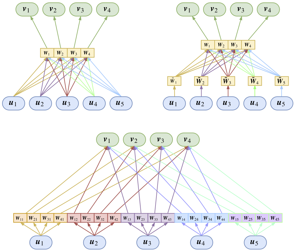Figure 4: Possible placements of Capsule's transformation matrices

Conclusion

Through these two rather sprawling (and somewhat rambling) posts, I've tried to work out an interpretation of the Capsule model that Hinton has been championing so vigorously. Given my own limited abilities, I ask readers' forgiveness for any inaccuracies.

Personally, I do believe Capsule is a genuinely novel and promising line of research. It may not turn out to be the future direction (though it certainly could be), but examining it closely still has much to teach us.

Looking back now at the goal I set out at the start of this post—trying to make Capsule feel a little more natural—I wonder how readers feel about it now? My own sense is that, after this kind of analysis, Capsule no longer feels quite so detached from everything else, but rather like a bold experiment: Hinton boldly folded the iterative process of clustering directly into a neural network, and out of that, Capsule was born.

Does that mean we might consider folding other intuitive algorithms into neural networks in similar ways, giving rise to other interesting creations? Let's wait and see.