SPACES: An "Extract-then-Generate" Approach to Long-Text Summarization (CAIL Competition Summary)

SPACES：“抽取-生成”式长文本摘要（法研杯总结） 苏剑林 · 2021-01-01 · Machine Learning text generation sparse text summarization

The "CAIL" (China AI and Law Challenge) is one of the more well-known NLP competitions in recent years. This year marks its third edition, comprising four tracks, one of which — "Judicial Summarization" — caught our attention. As we learned more, this track turned out to be about generating summaries for long legal judgment documents, which appears to be the first publicly available long-text generation task and dataset in China. Over the past year or so, we have been continuously investing in and exploring text generation, so we decided to use this track as a "touchstone" to test our research results. Fortunately, we ended up winning first place in this track by a narrow margin. Here, we'd like to summarize and share our competition model.

Competition leaderboard screenshot

In this competition, we stepped outside the pure "model-training-as-alchemy" mindset and improved model performance through fairly general new methods such as a novel Copy mechanism and Sparse Softmax. Overall, our model is quite simple and effective, and it can run end-to-end. We believe our results have some reference value for both engineering and research.more

Task Analysis

Observing and analyzing the task data is the first — and quite important — step in NLP, since it bears on our subsequent model choices as well as the direction of later improvements.

Statistics

The organizers provided a total of 9,484 annotated samples for this competition, in the form of (source text, summary) pairs. The original training data also came with some auxiliary annotations, but for the sake of generality we did not use this auxiliary information — so in principle our model applies to any supervised summarization task where each sample takes the form of a (source text, summary) pair.

Here are some statistics on the training data:

1. Total count: 9,484;
2. Input: average length 2,568 characters, standard deviation 1,122 characters, maximum 13,064 characters, minimum 866 characters;
3. Output: average length 283 characters, standard deviation 36 characters, maximum 474 characters, minimum 66 characters;
4. Metric: word-level weighted Rouge.

So, roughly speaking, this is a text generation task with "~3,000 characters in, ~300 characters out." The difficulty lies in the fact that an average length of over 2,000 characters far exceeds what we typically deal with. The 9,484 samples make up the full released dataset; the phase-1 data currently downloadable online contains 4,047 samples, and it's actually enough to get quite decent results. The model overall doesn't depend too heavily on data volume, so readers shouldn't worry too much about that.

Sample Preview

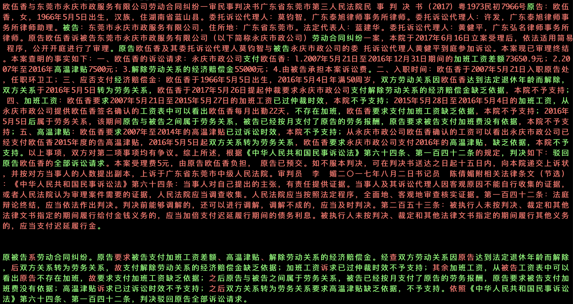Sample from the CAIL 2020 Judicial Summarization track

The image above shows a sample from the training set, where the top is the input (the original judgment document) and the bottom is the output (the human-annotated summary), with the green portions marking the "longest common subsequence" between the two. As you can see, the output overlaps heavily with the input.

Modeling Approach

Given these data characteristics, it's natural to consider a combined "extract + generate" approach to summarization, paired with some new techniques to ensure faithfulness of the summary and improve the final results. We named our final model SPACES:

S: Sparse Softmax (a newly designed replacement for Softmax);
P: Pretrained Language Model;
A: Abstractive (i.e., generative);
C: Copy Mechanism (a newly designed Copy mechanism);
E: Extractive;
S: Special Words (adding special words to the pretrained model).

Obviously, this is a "painstakingly" contrived acronym (facepalm), matching one of this blog's domain names, "spaces.ac.cn". Still, the acronym does list out the main technical points of our model. Below we'll go through what SPACES actually consists of in detail.

The Extraction Model

In this section we give a brief introduction to the extraction model component. The idea is to first use rules to convert the original generative-style corpus into a sequence-labeling corpus, and then model it with the DGCNN architecture that I frequently use.

Corpus Conversion

First, we need to keep in mind that the extraction model is only an intermediate step, not the final result — the extraction output still needs to be fed into the Seq2Seq model for further optimization. Therefore, the guiding principle for the extraction model is "completeness/recall": we want to cover as much of the information needed for the final summary as possible. To this end, we convert the original training corpus into an extractive corpus following these rules:

1. Build our own sentence-splitting function to achieve finer sentence granularity;
2. For each sentence in the human-written summary, find the most similar sentence in the source text (matches can repeat);
3. Use all matched source sentences as extraction labels;
4. Remove some of the matched sentences so as to maximize the Rouge score against the human summary.

Note that we removed step 4 in our final model, even though it was the default choice in our earliest version. In fact, adding step 4 improves the extraction model's own metrics, but after combining it with the generation model, the final score actually dropped. This is not hard to understand: the generation model already has the ability to delete and rewrite content, and it does this better than the extraction model. If the extraction model accidentally deletes a key sentence that should have been extracted, the generation model has a hard time recovering it, leading to a performance drop. In other words, step 4 violates the "completeness" principle of the extraction model — the job of deleting and rewriting should be left to the generation model, not baked into extraction.

The Metric Issue

The conversion process above involves choosing a "similarity" measure. As mentioned earlier, this competition uses "word-level weighted Rouge" as the evaluation metric, so we could naturally use this weighted Rouge directly as the similarity measure. Indeed, that's what we did at first, but during debugging we found this wasn't actually a good choice, and we ultimately switched to "character-level weighted Rouge."

What's the difference between the two? It's easy to see why the organizers chose to compute the metric at the word level: it ensures that proper nouns must match exactly. For example, suppose the ground truth is "PRC Law on the Protection of Minors" but your prediction is "PRC Law on the Protection of Cultural Relics." At the character level, the longest common subsequence would be "PRC ... Law on the Protection of ...", which still gets credit for most of it being correct. But at the word level, the two phrases are entirely different words, so it counts as completely wrong. So, word-level matching helps ensure that proper nouns are matched precisely.

However, word-level matching brings a serious side effect: it downweights long words/terms. For example, in "根据 《 中国人民共和国未成年人保护法 》 的 有关 规定" ("pursuant to the relevant provisions of the PRC Law on the Protection of Minors"), the core term "PRC Law on the Protection of Minors" only gets a weight of 1, while the remaining, largely unimportant words like "pursuant to", "《", "》", "的" each also get a weight of 1 — and together these make up the majority of the weight. As a result, the model would rather match trivial words like "pursuant to", "《", "》", "的" than fit the core term "PRC Law on the Protection of Minors." In short, with word-level scoring, a summary that scores high isn't necessarily one that captures the key information.

So how do we reconcile the two? In fact, the best approach would probably still be word-level matching, but weighting each word by its character count when computing the score — for instance, "PRC Law on the Protection of Minors" should get 0 points if unmatched, but 14 points (since it has 14 characters) rather than just 1 point if matched correctly. However, this would require implementing our own Rouge computation function, which is a bit of a hassle. In the end we simply chose character-level weighted Rouge, which turned out to be good enough in practice, since when converting the corpus, we know that the summary and source text are describing the same case, so situations like predicting "PRC Law on the Protection of Cultural Relics" instead of "PRC Law on the Protection of Minors" essentially don't arise.

Model Architecture

Back to the model itself: we use a sentence-level sequence-labeling model as the extraction model. Sentence embeddings are generated via "BERT + mean pooling" and kept fixed, while the labeling model itself is built with DGCNN. For more on DGCNN, see A CNN-based Reading-Comprehension-Style QA Model: DGCNN, Open-Sourcing a DGCNN Reading Comprehension QA Model (Keras version), and A Lightweight Information Extraction Model Based on DGCNN and Probabilistic Graphs.

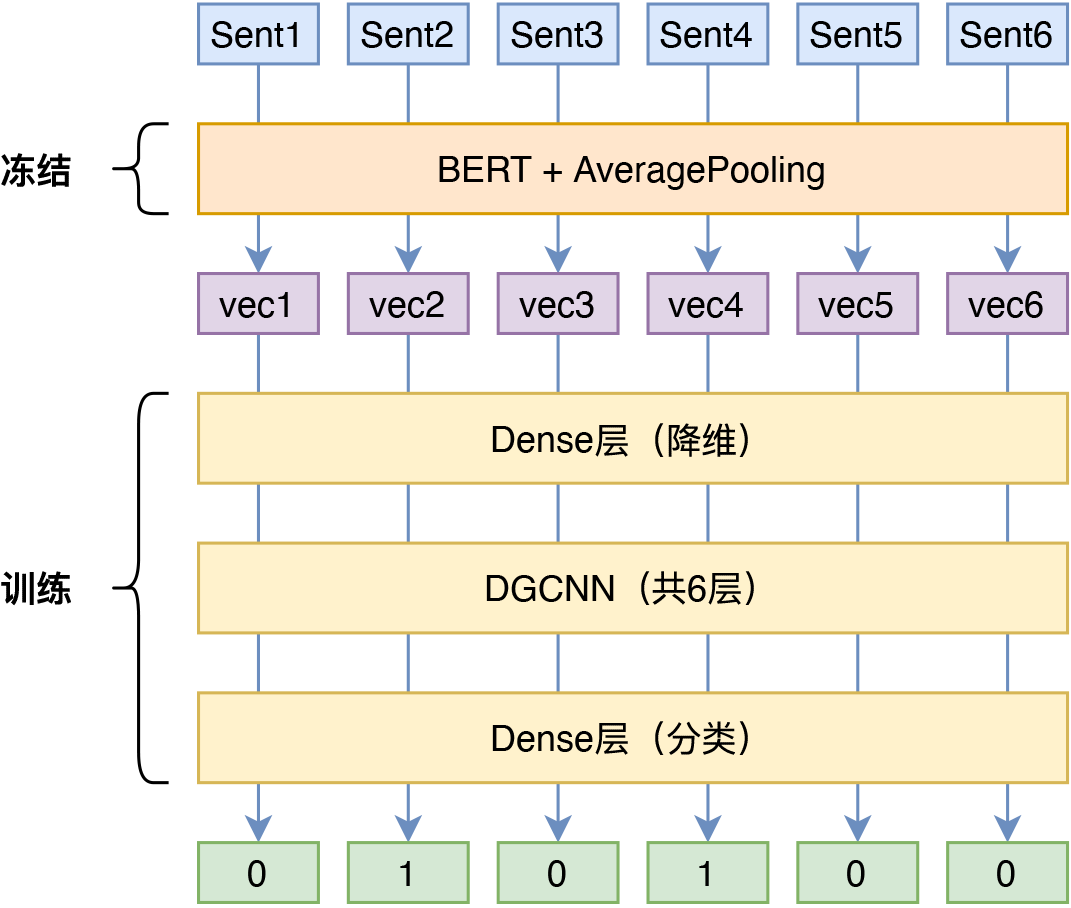Diagram of SPACES' extraction model

One detail worth pointing out: when training the extraction model, we used a threshold of 0.3 for early stopping, but ultimately used a threshold of 0.2 when constructing the data for the generation model — again following the "completeness" principle for the extraction model discussed above.

Producing the Output Data

We need to feed the source text into the extraction model to obtain an extractive summary, and then feed that extractive summary into the generation model to produce the final summary. But there's a subtlety here: the training data is data we've already seen, whereas at inference time we're dealing with unseen data. If we simply train an extraction model and then use it to extract summaries from the training set itself, the extraction scores on the training set will obviously be inflated (since the model has already seen this data), while performance on new samples will be lower — causing a train/inference mismatch.

The solution here is cross-validation. Specifically, we split the labeled data into $n$ folds, use $n-1$ of them to train the extraction model, and then use that model to predict extractive summaries for the remaining fold. Repeating this $n$ times gives us extractive summaries for the entire dataset, while minimizing the mismatch between training and inference.

The Generation Model

The generation model is where we invested most of our time, and it's our main contribution. The generation model is a Seq2Seq model trained with the extraction model's output as input and the human-annotated summary as the target — essentially, it performs further "polishing" of the extracted result.

Model Overview

Here's a diagram summarizing our generation model as a whole:

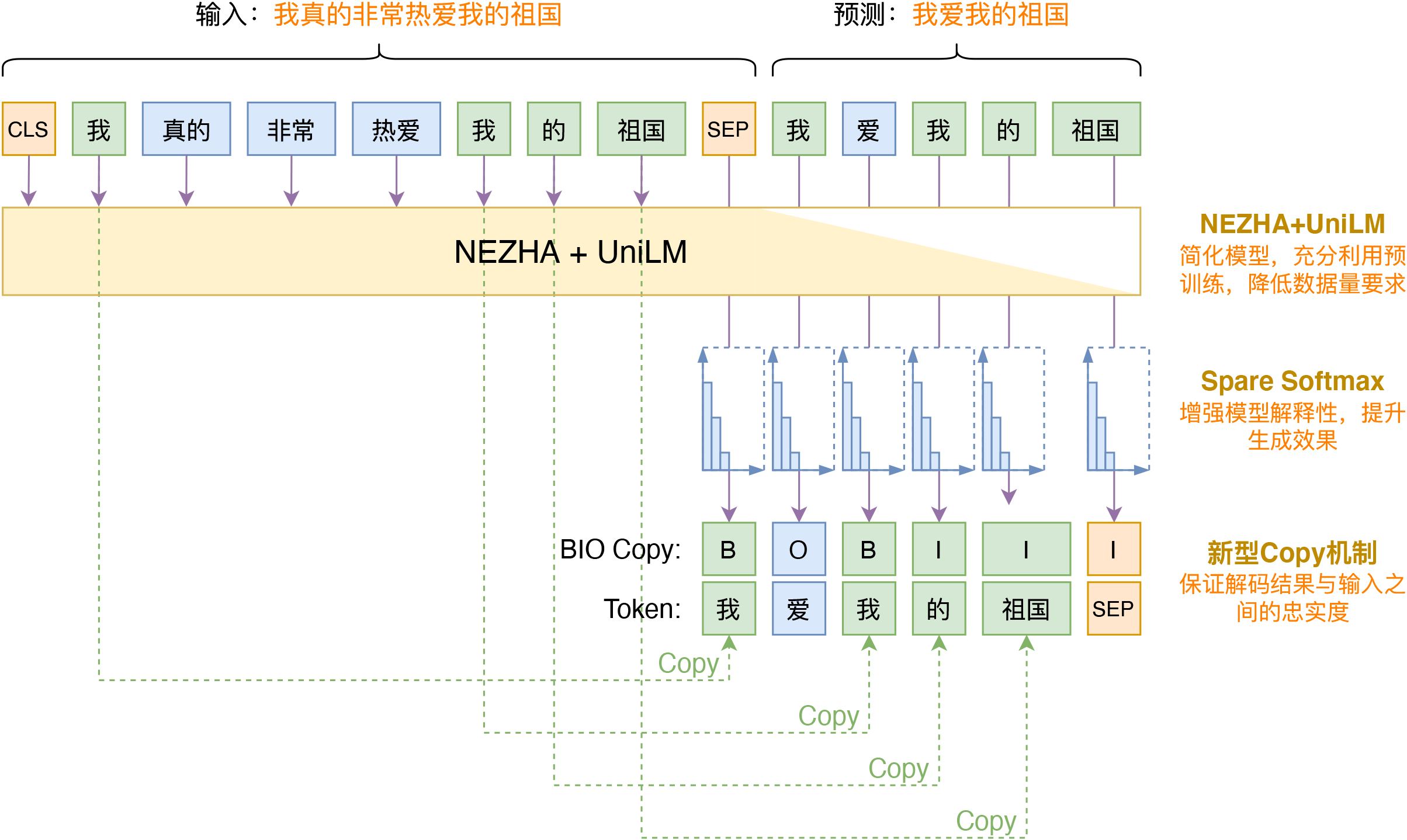Diagram of SPACES' generation model

Let's go through each module of the model.

Base Architecture

For the Seq2Seq model we again chose the classic UniLM approach (see From Language Models to Seq2Seq: Transformer as Theater, All Thanks to Masking), and since the combined length of "input + output" almost always exceeds 512, we chose Huawei's NEZHA model as the base architecture, since NEZHA uses relative position encoding and has no fixed length limit.

Of course, that was our choice at the time; nowadays we'd have at least two additional options:

1. Follow the approach in Hierarchically Decomposed Position Encoding: Letting BERT Handle Ultra-Long Text, which directly extends absolute position encoding, giving BERT the ability to directly handle much longer sequences (theoretically up to 260,000 tokens) — this can naturally be used within "BERT + UniLM" as well;
2. Use the multilingual T5 model (mT5) introduced in That Chart-Topping T5 Model Can Now Be Played With in Chinese, which also uses relative position encoding with no length limit — though note that T5's tokenizer converts full-width commas to half-width commas, which can hurt the evaluation score.

Additionally, in terms of using pretrained models, we were the first to incorporate certain words into the NEZHA model, breaking from the common practice of Chinese pretrained models operating at the character level — this brought some improvement in both effectiveness and speed. These results have already been published in an earlier post, Faster Without Losing Accuracy: Word-Granularity Chinese WoBERT, which readers can refer to.

BIO Copy

The Copy mechanism is nothing new in summarization models — it could even be called a standard component of abstractive summarization at this point. The conventional Copy mechanism generally follows Pointer Networks, but this approach has two shortcomings: 1) it can only copy one token at a time, with no guarantee of copying a contiguous span (n-gram); 2) it's relatively complex to implement and not very plug-and-play. To address this, we designed a new type of Copy mechanism, which we'll call BIO Copy for now — it's extremely simple to implement and is capable of copying contiguous spans.

Actually, the earlier diagram already illustrated this Copy mechanism. It essentially adds one more sequence prediction task on the Decoder side. Whereas the Decoder originally models the distribution over each token $p(y_t|y_{< t}, x)$, it now additionally predicts a label distribution, giving us

\begin{equation}p(y_t, z_t|y_{< t}, x) = p(y_t|y_{< t}, x) p(z_t|y_{< t}, x)\end{equation}

where $z_t\in\{\text{B},\text{I},\text{O}\}$, with the following meanings:

B: this token is copied from the source;
I: this token is copied from the source and forms a contiguous span together with the preceding token;
O: this token is not copied from the source.

So where do the labels $z$ come from during training? We use a fairly simple approach here: compute the "longest common subsequence" between the summary and the source text, and treat any token appearing in this longest common subsequence as having been copied, assigning it a B/I/O label according to the definitions above. For example, in the earlier illustration, the longest common subsequence between "我 真的 非常 热爱 我 的 祖国" and "我 爱 我 的 祖国" is "我 我 的 祖国," where the first "我" is a standalone character labeled B, and the following "我 的 祖国" forms a contiguous span labeled "B I I," with all other tokens labeled O — giving the overall label sequence "B O B I I."

So during training, this simply amounts to an additional sequence prediction task with fully known labels, which is easy to implement and adds essentially no extra computational cost. As for inference, at each step we first predict the label $z_t$: if $z_t$ is O, nothing changes; if $z_t$ is B, we mask out all tokens in the token distribution that don't appear in the source text; if $z_t$ is I, we mask out all tokens that would not form a valid n-gram matching the source text. In other words, decoding still proceeds step by step rather than generating an entire span at once, but through masking we can guarantee that the tokens at positions labeled B/I form an actual span from the source text.

It should be noted that introducing the Copy mechanism doesn't necessarily boost the score dramatically — as I recall, it only improved things by about 0.5%. But the Copy mechanism does help ensure the summary stays faithful to the original text and avoids professional/factual errors, which is quite important in practical use.

Sparse Softmax

In this competition, we also discovered a replacement for Softmax and cross-entropy, which we call Sparse Softmax. We found that Sparse Softmax can replace Softmax in quite a wide range of classification problems (including standard classification and text generation), typically yielding some improvement.

The idea behind Sparse Softmax draws on papers such as From Softmax to Sparsemax: A Sparse Model of Attention and Multi-Label Classification and Sparse Sequence-to-Sequence Models, where the authors proposed sparsifying Softmax to enhance interpretability and even improve performance. However, I found their designs a bit too complicated, so I came up with a simpler version myself:

$$\begin{array}{c|c|c} \hline & \text{original version} & \text{sparse version} \\ \hline softmax & p_i = \frac{e^{s_i}}{\sum\limits_{j=1}^{n} e^{s_j}} & p_i=\left\{\begin{aligned}&\frac{e^{s_i}}{\sum\limits_{j\in\Omega_k} e^{s_j}},\,i\in\Omega_k\\ &\quad 0,\,i\not\in\Omega_k\end{aligned}\right.\\ \hline 交叉熵 & \log\left(\sum\limits_{i=1}^n e^{s_i}\right) - s_t & \log\left(\sum\limits_{i\in\Omega_k} e^{s_i}\right) - s_t\\ \hline \end{array}$$

where $\Omega_k$ is the index set of the top $k$ elements when $s_1, s_2, \dots, s_n$ is sorted in descending order. In plain terms, our proposed Sparse Softmax, when computing probabilities, keeps only the top $k$ values and zeroes out the rest, where $k$ is a manually chosen hyperparameter — in this competition we used $k=10$. When computing cross-entropy, instead of summing over the entire set of classes $\text{logsumexp}$ as usual, we only sum over the top $k$ classes, where $t$ denotes the target class.

Why does sparsification help? We believe it's because it avoids the "over-learning" problem of Softmax. Suppose classification has already succeeded, i.e., $s_{\max}=s_t$ (the target class has the highest score). We can then derive an inequality for the original cross-entropy:

\begin{equation}\begin{aligned} \log\left(\sum\limits_{i=1}^n e^{s_i}\right)-s_{\max} &= \log\left(1+\sum\limits_{i\neq t} e^{s_i-s_{\max}}\right)\\ &\geq \log\left(1+(n-1) e^{s_{\min}-s_{\max}}\right) \end{aligned}\end{equation}

Suppose the current cross-entropy value is $\varepsilon$; solving gives

\begin{equation}s_{\max} - s_{\min}\geq \log (n-1) - \log \left(e^{\varepsilon} - 1\right) \end{equation}

Taking $\varepsilon=\ln 2=0.69...$ as an example, we get $\log \left(e^{\varepsilon} - 1\right)=0$, so $s_{\max} - s_{\min}\geq \log (n-1)$. In other words, in order to bring the loss down to 0.69, the gap between the largest and smallest logits must exceed $\log (n-1)$ — and when $n$ is large, this represents an unnecessarily large margin for a classification problem, since all we really need is for the target class's logit to be slightly larger than all non-target classes, not necessarily larger by as much as $\log (n-1)$. This means that regular cross-entropy is prone to over-learning and consequent overfitting, whereas truncation avoids this issue.

In this competition, Sparse Softmax may have brought about a 2% improvement (though we didn't measure it precisely). We've also privately run many additional experiments, both in NLP and CV, and found it gives roughly a 1% improvement on most tasks — so we'd definitely encourage everyone to try it! That said, we've also found that Sparse Softmax only works well in pretraining-based scenarios, since a pretrained model has already been trained thoroughly, so during fine-tuning the main concern is preventing overfitting. But if you're training a model from scratch, Sparse Softmax will actually hurt performance, since with only $k$ classes being learned from at each step, the model may end up under-trained (underfitting).

Other Details

When training the generation model, we incorporated EMA (exponential moving average of weights), which stabilizes training and can even improve model performance. In fact, EMA is more or less standard practice for me in competitions — it saves me a lot of effort in tuning the training schedule.

Also, regarding the BIO Copy mechanism: in principle, we only need to add a BIO prediction head on the Decoder side. However, in actual training, we added it on both the Encoder and Decoder sides, and found this improved the model's final performance. Intuitively, this likely works because adding it to both sides enhances the synchronization between Encoder and Decoder, helping guide the Decoder's attention to attend more precisely to the correct positions in the Encoder.

As for anything else worth adding, I'm still thinking — I'll add more if anything comes to mind.

Open-Source Release

The source code for the SPACES model has been released on GitHub:

SPACES: https://github.com/bojone/SPACES

Usage instructions are available on GitHub as well, so I won't repeat them here — feel free to open an issue or leave a comment if you have questions. Open-sourcing is a driving force behind technical progress, and whenever there are no conflicting interests, I try to open-source my work, and I encourage others to do the same.

Some readers might be curious about how good current automatic summarization can get, so here's a demonstration example (a validation set sample, with no manual edits; the first line is the source text, the second line is the reference summary, and the third line is the model-generated summary, with the green portions marking the longest common subsequence between the reference and model summaries):

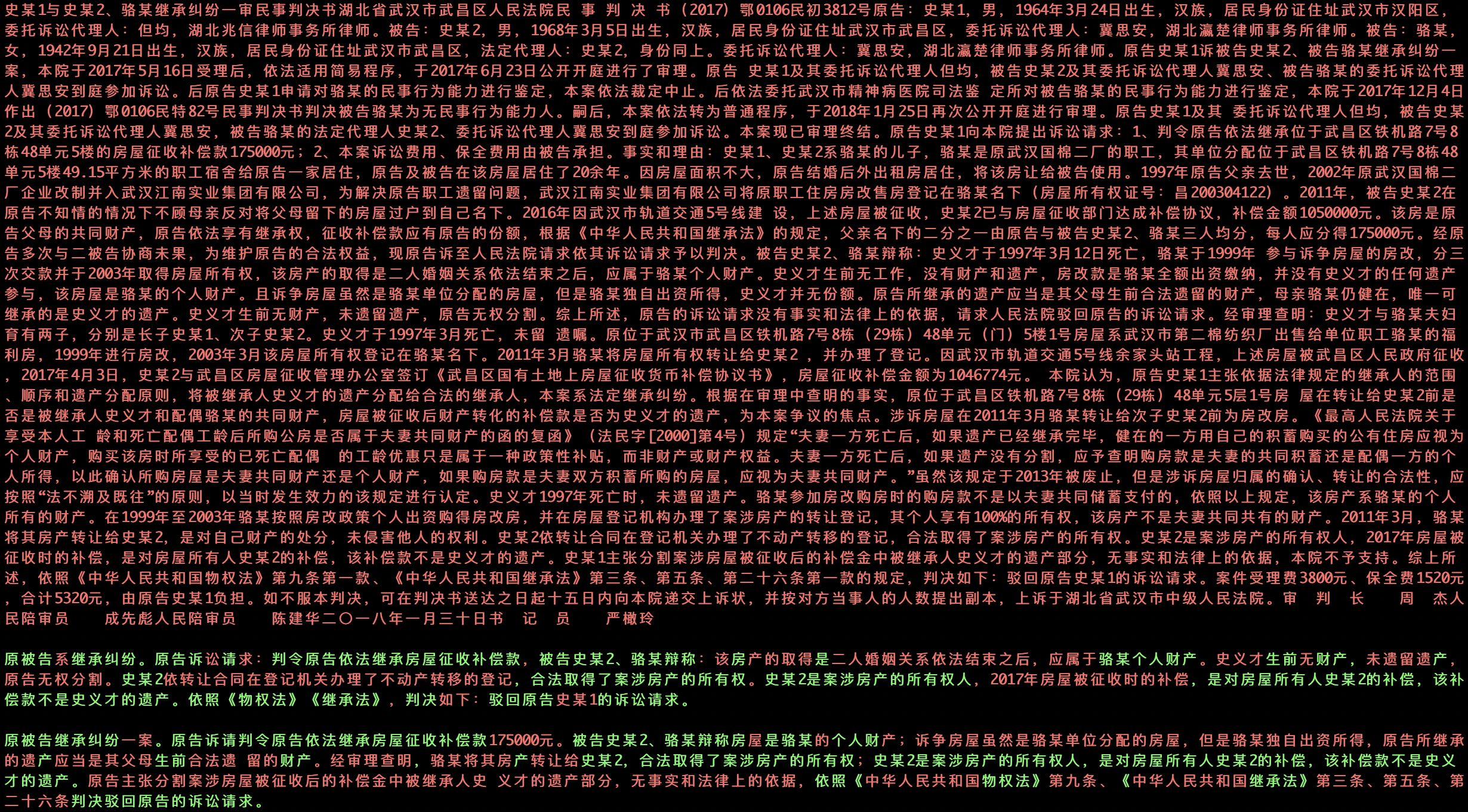Demonstration of final generation results (1)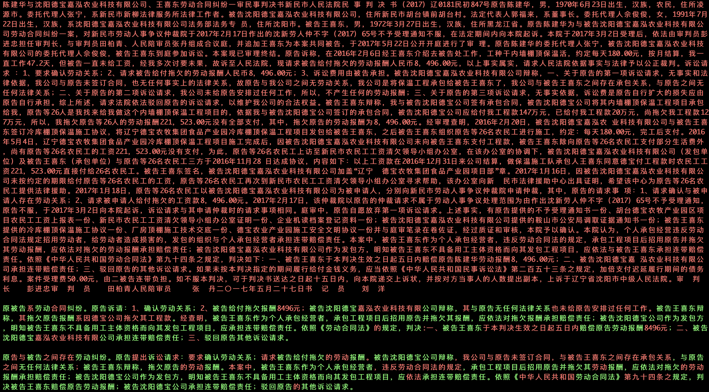Demonstration of final generation results (2)

Summary

This post summarized our approach to the CAIL judicial summarization task, presenting a long-text summarization model called SPACES. By adopting an "extract-then-generate" approach and combining our own BIO Copy mechanism, Sparse Softmax, and other methods, we were able to produce fairly reliable summaries. We welcome discussion and use of this approach.