CNN-Based Reading Comprehension QA Model: DGCNN
2019.08.20 Update: Open-sourced a Keras version (https://kexue.fm/archives/6906)
Back at the start of the year, in the introductory article on "Attention is All You Need", I already promised to share my experience with using CNNs in NLP, but somehow never got around to it. These past few days I finally made up my mind to write up the relevant material.
Background
Without further delay, let's first go over the basic setup of the model.
Model characteristics
This model — which I call DGCNN — is based on CNNs plus a simple form of attention. Since it doesn't use any RNN structure, it's remarkably fast, and since it's purpose-built for this WebQA-style task, it's also quite lightweight. The top models on the SQUAD leaderboard, such as AoA and R-Net, all rely on RNNs and are accompanied by fairly complex attention interaction mechanisms — none of which appear in DGCNN.
This is a model that can be trained in just a few hours even on a GTX1060!
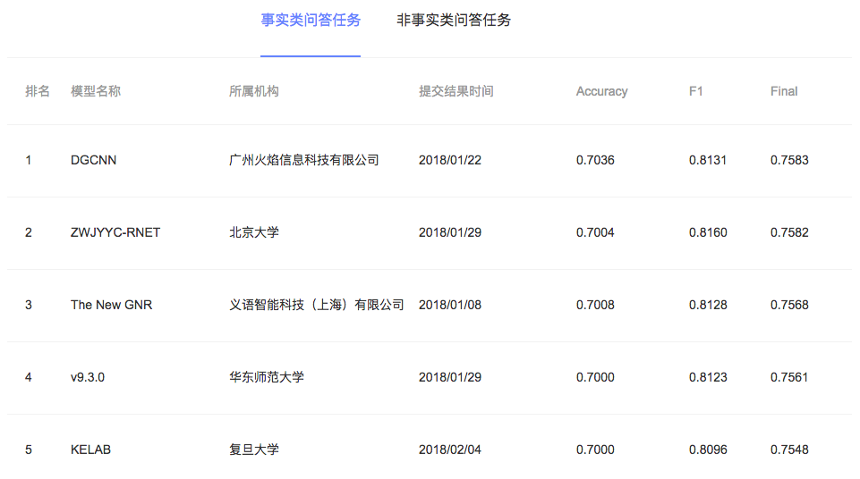 Leaderboard as of 2018.04.14
DGCNN, whose full name is Dilated Gated Convolutional Neural Network, combines two relatively new ways of using convolutions as its name suggests: dilated convolution and gated convolution, plus a handful of hand-crafted features and tricks, ultimately achieving the best performance while staying light and fast. At the time of writing, the model described here still sits at the top of the leaderboard, with a score (the average of accuracy and F1) of 0.7583, and is so far the only model that has never dropped out of the top three, while also having won the weekly championship the most times.
Competition context
This model was actually produced while I represented "Guangzhou Flame Technology Co., Ltd." in the CIPS-SOGOU QA competition. The competition started last October, but it's ended up a bit anticlimactic — even now it's stuck in limbo (no sign of ending, but also no sign of a new round starting).
In the first two or three months, competition was actually quite fierce — many companies and universities submitted models, and the leaderboard kept getting refreshed. So I feel it's a bit unfair to everyone who submitted with such enthusiasm for SOGOU to let it fizzle out like this. What's most frustrating is that there's never been any public announcement about their plans or changes, including the end date of the competition — contestants have just been left hanging. I later heard that the deadline is supposedly before this year's CIPS conference... a competition that runs for a whole year??
Brief description of the task
So far, SOGOU's competition has only run the "factoid" portion, and this factoid portion is basically the same format as the WebQA dataset that Baidu released earlier: "one question + multiple passages," where the goal is to jointly determine the precise answer to the question (usually an entity span) from multiple passages.
Question:
How many years of social security contributions are needed to receive a pension?
Answer:
15 years
Passage 1:
It's best not to quit; once you've paid in for 15 years, you can receive your pension upon retirement. If there's a special reason to quit, you can continue paying on your own.
Passage 2:
Hello! Once you've paid into the pension insurance for a full 15 years and reached retirement age, you can start receiving your pension.
Passage 3:
In everyday life, everyone pays into social security... how many years of contributions are needed to receive a pension upon retirement — the passage above has already explained this.
Compared with WebQA, the training set provided by Sogou is much noisier, which makes prediction harder. Moreover, I'd argue that this kind of WebQA-style task leans more toward retrieval matching and shallow semantic understanding, and is quite different from a similar overseas task like SQUAD (one long passage + multiple questions). In the SQUAD corpus, some questions involve fairly complex reasoning, which is why the top models on the SQUAD leaderboard tend to be more complex and larger in scale.
The Model
Now let's move on to the formal introduction of the model~
Architecture overview
Let's start with an overall diagram of the model.
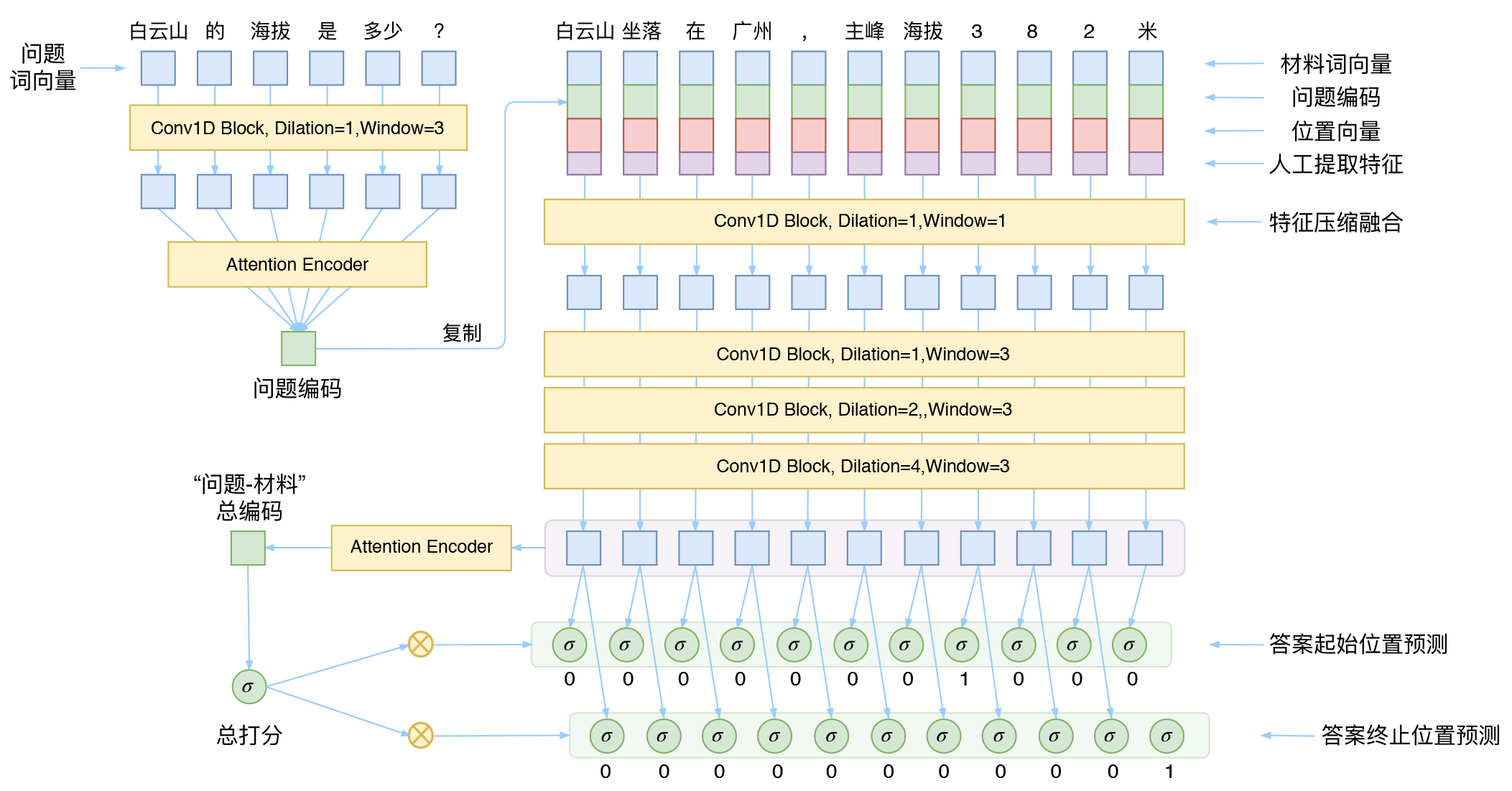 DGCNN model overview
As you can see from the diagram, for a "reading comprehension" / "QA system" model, this one is about as simple as it gets.
The overall architecture is derived from the WebQA reference paper Dataset and Neural Recurrent Sequence Labeling Model for Open-Domain Factoid Question. This paper has a few notable characteristics:
1. The question is directly encoded with an LSTM to produce a "question encoding," which is then concatenated onto every word vector of the passage;
2. Two hand-crafted co-occurrence features are extracted;
3. The final prediction is cast as a sequence labeling task, solved with a CRF.
DGCNN essentially follows this same line of thinking. Where we differ is:
1. All the LSTM components in the original model are replaced with CNNs;
2. We extract a richer set of co-occurrence features (8 of them);
3. We drop the CRF and instead use "0/1 labeling" to separately identify the start and end positions of the answer — this can be seen as a kind of "half-pointer, half-labeling" structure.
Convolutional structure
In this section we'll unpack the Conv1D Block shown in the diagram.
Gating mechanism
The convolutional structure used in the model comes from Facebook's Convolutional Sequence to Sequence Learning, and was also mentioned in my earlier post "Sharing a slide: fancy natural language processing". Suppose the vector sequence we want to process is $\boldsymbol{X}=[\boldsymbol{x}_1,\boldsymbol{x}_2,\dots,\boldsymbol{x}_n]$; we can add a gate to an ordinary 1D convolution as follows:
$$\boldsymbol{Y}=\text{Conv1D}_1(\boldsymbol{X}) \otimes \sigma\Big(\text{Conv1D}_2(\boldsymbol{X})\Big)\tag{1}$$
Note that here the two Conv1D layers have the same form (same number of filters, same window size, etc.), but their weights are not shared — meaning the parameter count is doubled. One of them is activated with a sigmoid function, the other has no activation at all, and the two outputs are multiplied element-wise. Since the sigmoid function's range is $(0,1)$, intuitively this amounts to adding a "valve" to each output of the Conv1D to control the flow. This is the GCNN structure — or, alternatively, we can regard this whole structure as an activation function, called GLU (Gated Linear Unit).
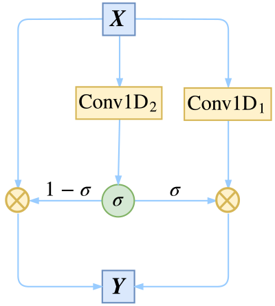 Combining residuals with gated convolution to achieve multi-channel transmission
Besides having an intuitive interpretation, one benefit of using GCNN is a lower risk of vanishing gradients, since one of the two convolutions has no activation function at all, and this unactivated part is less prone to gradient vanishing. When the input and output dimensions match, we can also add the input back in, i.e., use a residual structure:
$$\boldsymbol{Y}=\boldsymbol{X} + \text{Conv1D}_1(\boldsymbol{X}) \otimes \sigma\Big(\text{Conv1D}_2(\boldsymbol{X})\Big)\tag{2}$$
It's worth noting that we use the residual structure not merely to address vanishing gradients, but to allow information to flow through multiple channels. We can rewrite the equation above into an equivalent, more illustrative form, so we can see more clearly how information flows:
$$\begin{aligned}\boldsymbol{Y}=&\boldsymbol{X}\otimes \Big(1-\boldsymbol{\sigma}\Big) + \text{Conv1D}_1(\boldsymbol{X}) \otimes \boldsymbol{\sigma}\\ \boldsymbol{\sigma} =& \sigma\Big(\text{Conv1D}_2(\boldsymbol{X})\Big) \end{aligned}\tag{3}$$
From equation $(3)$ we can see the flow of information more clearly: with probability $1-\sigma$ it passes straight through, and with probability $\sigma$ it passes through only after being transformed. This form is very reminiscent of the GRU model in recurrent neural networks.
Supplementary derivation:
$$\begin{aligned}\boldsymbol{Y}=&\boldsymbol{X}\otimes \Big[1-\sigma\Big(\text{Conv1D}_2(\boldsymbol{X})\Big)\Big] + \text{Conv1D}_1(\boldsymbol{X}) \otimes \sigma\Big(\text{Conv1D}_2(\boldsymbol{X})\Big)\\ > =&\boldsymbol{X} + \Big(\text{Conv1D}_1(\boldsymbol{X}) - \boldsymbol{X}\Big)\otimes \sigma\Big(\text{Conv1D}_2(\boldsymbol{X})\Big) > \end{aligned}$$
Since $\text{Conv1D}_1$ has no activation function, it is simply a linear transformation, and so $\text{Conv1D}_1(\boldsymbol{X}) - \boldsymbol{X}$ can be merged together, effectively becoming a single $\text{Conv1D}_1$. In other words, during training, whatever $\text{Conv1D}_1(\boldsymbol{X}) - \boldsymbol{X}$ can achieve, $\text{Conv1D}_1(\boldsymbol{X})$ can also achieve. Hence $(2)$ and $(3)$ are equivalent.
Dilated convolution
Next, in order to let the CNN model capture longer-range dependencies without increasing the number of parameters, we use dilated convolution.
The contrast between ordinary convolution and dilated convolution can be illustrated with a single diagram:
 Ordinary convolution vs. dilated convolution
Consider a three-layer convolutional network (with the first layer being the input layer), with a window size of 3. With ordinary convolution, by the third layer each node can only capture 3 inputs to either side, having no connection at all to anything beyond that.
With dilated convolution, however, by the third layer each node can capture 7 inputs to either side, while the parameter count and speed remain unchanged. This is because at the second convolutional layer, the dilated convolution skips over the directly adjacent inputs and instead reaches straight to the center and its second-nearest neighbors (a dilation rate of 2) — this can also be thought of as "a window of size 5 with two positions hollowed out." That's why dilated convolution is also called atrous convolution. At the third convolutional layer, it skips three consecutive inputs (a dilation rate of 4), which can likewise be seen as "a window of size 9 with 6 positions hollowed out." If you draw lines connecting the relevant inputs and outputs, you'll find that any given node at the third layer is connected to 7 original inputs on either side.
Following the principle of "as little overlap and omission as possible," the dilation rates of a dilated convolution generally grow as a geometric sequence: 1, 2, 4, 8, .... Note the phrase "as little as possible" — there is still some overlap. This scheme is borrowed from Google's WaveNet model.
Block
Now we can explain each Conv1D Block shown in the model diagram: when the input and output dimensions match, it is the dilated-convolution version of equation $(3)$; when the input and output dimensions don't match, it is simply equation $(1)$. The window sizes and dilation rates are all labeled in the diagram.
Attention
As shown in the model diagram, in this DGCNN model, attention is mainly used in place of simple pooling to aggregate sequence information — both for encoding the question's vector sequence into a single overall question vector, and for encoding the passage's sequence into a single overall passage vector. The attention used here is slightly different from the attention in Attention is All You Need; the attention used in this post can be regarded as a form of "additive attention," with the form
$$\begin{aligned}\boldsymbol{x}&=\text{Ecndoer}\big(\boldsymbol{x}_1,\boldsymbol{x}_2,\dots,\boldsymbol{x}_n\big)=\sum_{i=1}^n \lambda_i \boldsymbol{x}_i\\ \lambda_i&=\mathop{\text{softmax}}_i\Big(\boldsymbol{\alpha}^{\top}\,\text{Act}\big(\boldsymbol{W}\boldsymbol{x}_i\big)\Big)\end{aligned}\tag{4}$$
Here, $\boldsymbol{\alpha},\boldsymbol{W}$ are all trainable parameters, and $\text{Act}$ is an activation function, typically taken to be $\tanh$, though $\text{swish}$ could also be considered. Note that when using $\text{swish}$, it's best to also include a bias term, giving
$$\lambda_i=\mathop{\text{softmax}}_i\Big(\boldsymbol{\alpha}^{\top}\,\text{Act}\big(\boldsymbol{W}\boldsymbol{x}_i+\boldsymbol{b}\big)+\beta\Big)\tag{5}$$
This attention scheme is borrowed from the R-Net model. (Note: it may not have originated with R-Net — I simply learned it from R-Net.)
Position vectors
To strengthen the CNN's sense of position, we also add position vectors, concatenated onto each word vector of the passage. The construction of the position vectors directly follows the scheme in Attention is All You Need:
$$\left\{\begin{aligned}&PE_{2i}(p)=\sin\Big(p/10000^{2i/{d_{pos}}}\Big)\\ &PE_{2i+1}(p)=\cos\Big(p/10000^{2i/{d_{pos}}}\Big) \end{aligned}\right.\tag{6}$$
Output design
This part is one of the more distinctive aspects of our overall model.
Design rationale
By this point, the overall structure of the model should already be clear. First, we use convolution and attention to encode the question into a fixed vector; this vector is concatenated onto every word vector of the passage, along with the position vectors and hand-crafted features. At this point we have a feature sequence that mixes together information from both the question and the passage, and we can process this sequence directly — so we follow it with a few more convolutional layers for further encoding, and then label the sequence directly, with no need for further interaction with the question.
In the SQUAD evaluation, the passage is guaranteed to contain an answer, and the location of that answer is fully annotated, so SQUAD models typically apply softmax twice over the whole sequence to predict the start and end positions of the answer — commonly called a "pointer network." However, in our WebQA-style QA setting, the passage may not contain an answer at all, so instead of softmax we apply sigmoid across the entire sequence. This both allows for the possibility that the passage has no answer, and allows the answer to appear multiple times within the passage.
Dual-labeling output
Given that we're using labeling, in principle the simplest approach would be to output a single 0/1 sequence: directly labeling each word in the passage as "yes (1)" or "no (0)" for being part of the answer. However, this doesn't work very well in practice, because an answer may consist of several consecutive but different words, and forcing the model to assign the same label to all of these different words can be "asking too much" of the model. So instead we use two rounds of labeling, to separately mark the start and end positions of the answer.
$$\begin{aligned}p^{start}_i = \sigma\Big(\boldsymbol{\alpha}_1^{\top}\,\text{Act}\big(\boldsymbol{W}_1\boldsymbol{x}_i+\boldsymbol{b}_1\big)+\beta_1\Big)\\ p^{end}_i = \sigma\Big(\boldsymbol{\alpha}_2^{\top}\,\text{Act}\big(\boldsymbol{W}_2\boldsymbol{x}_i+\boldsymbol{b}_2\big)+\beta_2\Big)\end{aligned}\tag{7}$$
In this way, the output design of the model is neither purely a pointer-network approach nor purely sequence labeling — it's more like a simplified fusion of the two.
The big picture
Finally, to give the model more of a "global perspective," we encode the material's sequence into a single overall vector, then apply a fully connected layer to obtain a global score, and multiply this score into the labels computed earlier, turning it into
$$\begin{aligned}\boldsymbol{o}=&\text{Ecndoer}\big(\boldsymbol{x}_1,\boldsymbol{x}_2,\dots,\boldsymbol{x}_n\big)\\ p^{global}=&\sigma\Big(\boldsymbol{W}\boldsymbol{o}+\boldsymbol{b}\Big)\\ p^{start}_i =& p^{global}\cdot\sigma\Big(\boldsymbol{\alpha}_1^{\top}\,\text{Act}\big(\boldsymbol{W}_1\boldsymbol{x}_i+\boldsymbol{b}_1\big)+\beta_1\Big)\\ p^{end}_i =& p^{global}\cdot\sigma\Big(\boldsymbol{\alpha}_2^{\top}\,\text{Act}\big(\boldsymbol{W}_2\boldsymbol{x}_i+\boldsymbol{b}_2\big)+\beta_2\Big)\end{aligned}\tag{8}$$
This global score is important for the model's convergence and performance. Its purpose is to help the model better judge whether an answer even exists in the material — once it's clear the material contains no answer, we can simply set $p^{global}=0$, rather than "painstakingly" forcing every word's label to zero.
Handcrafted features
Earlier in the article, we already mentioned handcrafted features several times — so how much do they actually help? Based on a rough eyeball estimate, these few handcrafted features may boost model performance by more than 2%! This shows that well-designed features play an important role both in improving model performance and in reducing model complexity.
The handcrafted features are designed around the words in the material (Q stands for question, E stands for evidence, i.e., the material).
Q-E exact match
This checks whether a word in the material also appears in the question: 1 if it does, 0 if not. The idea behind this feature is to directly tell the model where the question's words show up in the material, since answers are likely to be located near those spots. This matches how humans approach reading comprehension.
E-E co-occurrence
This feature computes, for a given word in one piece of material, the proportion of other materials in which that word also appears. For example, suppose there are 10 passages, and a word w appears in the first passage; if w also appears in 4 of the remaining 9 passages, then word w in the first passage gets a handcrafted feature value of 4/10.
The idea here is that the more materials a word appears in, the more likely it is to be part of the answer.
Q-E soft match
Using the question's length as a window size, we compute the Jaccard similarity and relative edit distance for every window in the material.
For example, take the question "白云山 的 海拔 是 多少 ?" ("What is the elevation of Baiyun Mountain?"), and the material "白云山 坐落 在 广州 , 主峰 海拔 3 8 2 米" ("Baiyun Mountain is located in Guangzhou; its main peak has an elevation of 382 meters"). The question has 6 words, so the window size is 6. We split the material as follows:
X X X
白云山
坐落 在
X X 白云山
坐落
在 广州
X 白云山 坐落
在
广州 ,
白云山 坐落 在
广州
, 主峰
坐落 在 广州
,
主峰 海拔
在 广州 ,
主峰
海拔 3
广州 , 主峰
海拔
3 8
, 主峰 海拔
3
8 2
主峰 海拔 3
8
2 米
海拔 3 8
2
米 X
3 8 2
米
X X
Here X denotes a placeholder. With this split, we can compute the Jaccard similarity between each window and the question, and use this similarity score as a feature for the current word (shown in red in the original). For the example above, this gives [0.13, 0.11, 0.1, 0.09, 0.09, 0.09, 0.09, 0.09, 0.09, 0.1, 0].
Similarly, we can compute the edit distance between each window and the question, then divide by the window size to get a number between 0 and 1, which I call the "relative edit distance." For the example above, this gives [0.83, 0.83, 0.83, 0.83, 1, 1, 1, 0.83, 1, 1, 1].
Jaccard similarity is order-agnostic, while edit distance is order-sensitive, so these two approaches measure the similarity between the question and the material from complementary — order-agnostic and order-sensitive — perspectives. The idea behind these two features is the same as the first one: tell the model which part of the material resembles the question, since the answer is likely to be nearby.
The main idea behind these two features came from a member named Yin in the Keras group — thanks to him for that!
Character-level features
Nearly all of the top-ranking models on SQuAD feed both word embeddings and character embeddings into the model, and to boost performance we too would like to feed in character embeddings alongside word embeddings. But we didn't want to make the model too large, so instead we incorporated character-level features as part of our handcrafted features.
The idea is actually quite simple: the four features described above are all computed at the word level. In fact, we can compute them at the character level as well, then average the results of the characters within each word to get a character-level feature for that word. For instance, in the "Q-E exact match" feature: suppose the question contains only the word "演" ("perform"), while the material contains the word "合演" ("co-star"). At the word level, "合演" doesn't appear in the question, so the co-occurrence feature is 0. But if we look at characters instead, "合演" is split into two characters, "合" and "演." Computing the co-occurrence feature the same way, "合" gets 0 and "演" gets 1; averaging these gives 0.5, which becomes the character-level "Q-E exact match" feature for the word "合演."
The other three features are handled the same way, giving us four more features — for a total of 8 handcrafted features.
Implementation
By now, essentially every part of the model has been explained. Really, the model as a whole is simple and clear, and easy to describe — it should give a sense of "great truths are simple." Below, we cover some implementation details.
Model configuration
Here are some basic points about how the model was implemented.
Chinese word segmentation
As can be seen from the discussion above, this model operates on words, with character-level information introduced only lightly through the handcrafted features described earlier. However, to keep the model flexible enough to handle a wider variety of questions, we only applied a basic word segmentation to the input, aiming to keep the segmentation granularity as fine as possible.
Specifically: we wrote our own segmentation module based on a unigram model, using a self-prepared dictionary of roughly 500,000 words, while all English letters and digits were split into individual characters — for example, "apple" becomes five "words": a p p l e, and "382" becomes three "words": 3 8 2.
Since there's no new-word discovery mechanism, the entire vocabulary never exceeds 500,000 words. In fact, the final model ended up with a vocabulary of only about 300,000 words.
Of course, readers could also use Jieba segmentation, disabling its new-word discovery feature and manually splitting digits and English letters — the effect would be the same.
Some hyperparameters
1. Word embeddings are 128-dimensional, pretrained via Word2Vec on the competition's training corpus, the WebQA corpus, 500,000 Baidu Baike entries, and 1,000,000 Baike Zhidao questions. The Word2Vec model used Skip-Gram with a window size of 5, 8 negative samples, and 8 iterations; training took about 12 hours.
2. Padding tokens are represented by all-zero vectors, and word embeddings are kept fixed throughout the DGCNN model's training.
3. All Conv1D layers have an output dimension of 128, and the positional embeddings are also 128-dimensional.
4. The maximum sequence length is set to 100; whenever a batch contains samples requiring padding, the padded portions must be properly masked.
5. Since the task ultimately reduces to a binary labeling problem, and given the class imbalance between positive and negative labels, we use binary focal loss as the loss function.
6. Training uses the Adam optimizer: first train to convergence with a learning rate of $10^{-3}$ (roughly within 6 epochs), then load the best checkpoint and continue training to convergence with a learning rate of $10^{-4}$ (within 3 epochs).
Regularization term
Toward the later stages of the competition, we found a form of regularization similar to DropPath that gave a slight performance boost — though I'm not entirely sure how large the boost was; in any case, it did help at the time.
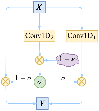 Perturbing the gates of the GCNN as a regularization term for the model
This regularization technique builds on equation $(3)$. The idea is to perturb the "gate" during training:
$$\begin{aligned}\boldsymbol{Y}=&\boldsymbol{X}\otimes \Big(1-\boldsymbol{\sigma}\Big) + \text{Conv1D}_1(\boldsymbol{X}) \otimes \boldsymbol{\sigma}\\ \boldsymbol{\sigma} =& \sigma\Big(\text{Conv1D}_2(\boldsymbol{X})\otimes (1 + \boldsymbol{\varepsilon})\Big) \end{aligned}\tag{9}$$
where $\boldsymbol{\varepsilon}$ is a tensor of uniform random numbers drawn from $[-0.1, 0.1]$. In this way, we introduce "multiplicative noise" into the GCNN's "gate," making the model more robust to small perturbations in its parameters.
This regularization scheme was, to some extent, inspired by the regularization techniques in FractalNet: Ultra-Deep Neural Networks without Residuals and Shake-Shake regularization.
Data preparation
Data preprocessing
Since the SOGOU competition allowed the use of external data, we — like most participating teams — supplemented training with the WebQA dataset. Since the WebQA dataset is relatively clean while the corpus provided by SOGOU is noisier, we mixed the SOGOU and WebQA corpora in a 2:1 ratio.
Both WebQA and SOGOU provide data in the form of "one question + multiple passages of material + one answer," without explicitly indicating which passage, or which position within a passage, the answer comes from. So we had no choice but to treat every substring in the material that exactly matches the answer as a possible answer location. For some samples this isn't entirely reasonable, but without additional manual annotation, this was the best we could do.
There's also the issue of synonyms between the training corpus's questions and answers — for example, when asked "Who plays Mr. Bean?" the standard answer is "Rowan Atkinson" (罗温艾金森), but the material might contain not just that exact string but variants like "罗温·艾金森," "罗温.艾金森," or "洛温·艾金森" (alternate transliterations/spellings). One nice thing about the SOGOU competition is that it provided a fairly objective offline evaluation script, and this script accounts for synonym variation — so we were able to extract answer synonyms from the evaluation script itself and use them to label all equivalent answers.
There were also some operations like converting full-width characters to half-width, which readers will naturally think of once they look at the dataset, so we won't go into detail here.
Data shuffling
In the end, SOGOU provided annotated data for 30,000 questions, with a pre-split training set (25,000) and validation set (5,000). But if we trained directly using this split, the validation set's structure diverged noticeably from the results we got on the official leaderboard.
So instead, we pooled all the annotated data, shuffled it, and re-split it into a training set (20,000) and validation set (10,000). This gave a validation score of about 0.76, close to the leaderboard result.
Data augmentation
During training, we used three operations that could be considered forms of data augmentation.
1. Randomly zeroing out some word IDs in the question and material: both the question and the material are fed in as sequences of word IDs, with 0 serving as the padding token (equivalent to a mask). Randomly zeroing out words means randomly replacing them with the padding token, which reduces the model's dependence on any particular word.
2. Generating new material by repeatedly concatenating and then randomly cropping the same passage (this also changes the number and positions of the answers accordingly).
3. For material where the answer appears multiple times, randomly dropping some of the answer annotations. For instance, if the answer "Guangdong" appears twice in a passage, when labeling the answer we might label only the first occurrence, only the second, or both.
From what I recall, the first augmentation technique had the biggest impact, effectively improving both the stability and accuracy of the model, while the second and third were comparatively weaker. The difference between the first augmentation technique and simply applying dropout to the word embedding sequence is that dropout, besides randomly zeroing values, also rescales the remaining values — whereas here we deliberately avoid that rescaling, which makes the operation easier to interpret.
Decoding strategy
One detail that many competitors may have overlooked is: there can be a lot of room to optimize how the answer is decoded, and the gains from optimizing decoding may far exceed the gains from repeatedly tuning the model's hyperparameters!
Scoring method
What exactly is answer decoding? Whether using a softmax-style pointer network or the sigmoid-based "half-pointer, half-labeling" approach described in this article, the model's final output consists of two columns of floating-point numbers, representing the scores for the start position and the end position of the answer, respectively. But the question is: what metric should be used to determine the answer span? The usual approach is: fix a maximum answer length, max_words (I used 10, counting each Chinese character as 1 and each letter/digit as 0.5), then enumerate all spans in the material no longer than max_words, compute the sum or product of their start and end scores, and take the maximum. So here's the question: is "sum" better, or "product"? Or perhaps the "square root of the product"?
At first I went with intuition and felt that "square root of the product" was the most sensible choice. Later, I tested switching directly to "product" and found the performance improved noticeably (by about 1%). This led me to reconsider this decoding decision more carefully, and I discovered that there are actually quite a few pitfalls here — this decoding choice is itself an important hyperparameter, and shouldn't be decided purely by intuition.
Voting method
For example, when the same span of text appears multiple times within the same passage, should we sum the scores of those occurrences, average them, or just take the maximum? And once every passage has produced its own candidate answer, how do we combine the answers from all these passages into a final voted answer?
Suppose we have 5 passages, and the answers and scores they each produce are (A, 0.7), (B, 0.2), (B, 0.2), (B, 0.2), (B, 0.2) — should the final output be A or B? Some might say "three cobblers with their wits combined equal a master strategist" — where the "cobblers" here refer to the low-scoring answer B, and the "master strategist" refers to the high-scoring answer A. Since the four B scores sum to 0.8 > 0.7, it might seem like we should output B.
I don't think that's quite right. In real life, an expert is not simply equivalent to a pile of ordinary people — there's strength in numbers, sure, but often $1+1$ ends up smaller than $2$. Take the answer distribution above: intuitively, we'd actually prefer to pick answer A, because it's close to a perfect score of 1 and clearly stands out relative to the other answers.
So our voting scheme needs to embody two principles: 1) there's strength in numbers; 2) $1+1 < 2$. This rules out both simple summation and simple averaging. The simplest scheme that works is a "sum of squares":
1. For the same passage, if a given span appears multiple times, we take only the maximum score among them — we don't average or sum — because "the same passage" is effectively "the same person," and there's no need to let one person's vote count multiple times.
2. After this step, each passage has "elected" its own answer — each passage now acts like a single "cobbler" or "master strategist," and each answer carries a score representing that cobbler's or strategist's decision. We then take the "sum of squares" of the scores of identical answers as that answer's final score, and pick the answer with the largest final score among all distinct answers:
$$s_a = \sum_{i=1}^n s^2_{a,i}$$
This is because "squaring" amplifies the weight of higher-scoring samples.
3. Compared to step 2, in the competition I actually used a slightly different scoring formula:
$$s_a = \frac{\sum\limits_{i=1}^n s^2_{a,i}}{1+\sum\limits_{i=1}^n s_{a,i}}$$
This formula follows the same "sum of squares" idea, but takes an additional average, with a "+1" added to the denominator. The "squaring" operation weights the experts more heavily, while the "+1" penalizes small sample counts — this formula is gentler overall than a plain sum of squares.
Note that it wasn't just our model that benefited from this — when I discussed this with another competitor and suggested this decoding approach to them, they applied the same idea after some tuning and also saw a substantial improvement.
Model Ensembling
After following the steps above, the model should reliably score around 0.74–0.75 on SOGOU's online test set. But to reach the optimal 0.7583, model ensembling is needed.
Model ensembling can be divided into single-model ensembling and multi-model ensembling. Single-model ensembling means training the same model architecture multiple times in different ways and then averaging the results; multi-model ensembling means doing a single-model ensemble for each of several different models, and then ensembling those single-model ensemble results together. For simplicity, we only did single-model ensembling.
Single-model ensembling is built on top of cross-validation. As mentioned earlier, we shuffled the labeled corpus and re-split it into training and validation sets; a more thorough approach is cross-validation, where the shuffled labeled corpus is split into $k$ folds, and each fold is used once as the validation set (each time requiring the model to be trained from scratch):
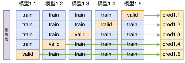 k-fold cross-validation of the model
This gives us $k$ different training results for the same model, and averaging these results is what constitutes model ensembling:
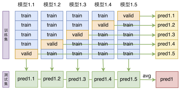 Single-model ensembling based on cross-validation
Afterword
Performance Evaluation
The leaderboard speaks for itself, so the model's performance is there for all to see. On SOGOU's closed test set, which has quite a lot of noise, our model ultimately scored 0.7583. And looking at the training set, I suspect some of the noise was deliberately introduced—some of the materials are so absurd that even directly pulling a batch of results from a search engine or Baidu Zhidao wouldn't be that bad. So I believe the model would perform even better in actual use. Combined with the fact that it's a lightweight, pure-CNN model, this fully meets industrial requirements.
I also tested this model on SQUAD, and found the accuracy to be around 50%, though without fine-tuning or ensembling. With optimization and tuning, I'd estimate it could reach 60%+ accuracy. This is obviously quite far from the 0.7583 score, which also shows that WebQA-style reading comprehension QA is quite different from pure SQUAD-style reading comprehension, even though in theory the models are interchangeable.
Code & Testing
The model has been deployed on Firebird Technology's official website, and you can test it online by clicking this link:
http://www.birdbot.cn/online-factual-qa.html
(Mobile access may not work well; please try to access it from a PC. ^_^)
As for the code, I won't be open-sourcing it, for two reasons. First, this competition was entered on behalf of the company, so it's not appropriate to open-source everything directly—and besides, the model is genuinely simple and clear; after reading this article, it shouldn't be hard to implement it yourself. If readers still can't implement it after reading this, I'd suggest building up your coding fundamentals before diving into reading comprehension and QA systems. Second, once code is open-sourced, there are always some readers who don't even want to read the article—they just download the code directly, and then when it doesn't run, they bombard you with a stream of questions like "how do I install this library?" or "why is this line throwing an error?"—it's simply too much to keep up with.
This article is, after all, not meant to be a beginner's tutorial, so please forgive me. Of course, I don't mean to look down on beginners—the blog does occasionally feature beginner-level posts—just not this one.
Also, as a decent competitor, I can't directly share SOGOU's training corpus either. Readers who want to test this themselves can just train using the WebQA dataset.
Countless Trials and Tweaks
Finally, let me show you a screenshot:
Hundreds of search debugging attempts
This screenshot basically represents my entire debugging process, including hundreds of iterations of tuning, with multiple experiments run for every update—this has been the competition I've thrown myself into the most so far.
So, although this is not a formal paper, if readers genuinely gained something from it, I'd appreciate a citation of this article.
Last but not least, thanks to Guangzhou Firebird Technology for their support in both software and hardware—the company has given me a very friendly opportunity for growth and development.
PS: I later discovered that the model in this article actually "collides" with the two papers Fast Reading Comprehension with ConvNets and QANET: Combining Local Convolution with Global Self-Attention for Reading Comprehension. But when I was working on this competition, I genuinely had never referenced either of these two papers. At the time, I started from the WebQA paper, intending to reproduce the WebQA model, then got curious and wanted to try a CNN model instead—and things just took off from there.
Translated automatically with claude-sonnet-5; all equations are reproduced verbatim from the source. Copyright remains with the original author.