GAN Through the Lens of Energy (I): GAN = "Digging Pits" + "Jumping into Pits"

能量视角下的GAN模型（一）：GAN＝“挖坑”＋“跳坑” 苏剑林 · 2019-01-30 · Machine Learning probability energy GAN generative model

"Look at that pit-digger, what's different about him~"

In this series, we try to understand GANs from an energy perspective. We'll find this viewpoint to be so elegant and intuitive that it's genuinely striking.

This perspective is directly inspired by a new paper from Bengio's team, Maximum Entropy Generators for Energy-Based Models, which appeared on arXiv a few days ago. Of course, the connection between energy-based models and GANs has a long history and isn't an original contribution of this paper — it's just that this paper works it out especially carefully and thoroughly. This post also adds some of my own understanding and reflections on top, in an effort to make it more accessible and complete.

As the first post in the series, let's start with a plain analogy-based derivation: a GAN is really just a saga of "digging pits" and "jumping into pits", carried out in relentless succession (dig first, then jump?).

Broadly, here's what this post covers:

1. Gives a clear, intuitive energy picture of GAN/WGAN;
2. Discusses the training situation and strategy for the discriminator (the energy function);
3. Points out a beautiful and intuitive energy-based interpretation of gradient penalty;
4. Discusses the choice of optimizer in GAN training.

Dig First, Jump Later

In this section, we'll try to use as plain an analogy as possible to explain what GAN looks like from an energy perspective.

Suppose we have a batch of samples $x_1,x_2,\dots,x_{n}$, and we want to find a generative model capable of producing a batch of new samples $\hat{x}_1,\hat{x}_2,\dots,\hat{x}_{n}$ that closely resemble the original samples. How do we do this? It's simple — two steps.

"Digging Pits"

Step one, digging pits: we treat the real samples $x_1,x_2,\dots,x_{n}$ as a set of coordinates, and dig a bunch of pits at these coordinates. The distribution of these pits can be described by an energy function $U(x)$. This way, the real samples $x_1,x_2,\dots,x_{n}$ end up sitting at the bottom of the pits. Then we place the fake samples $\hat{x}_1,\hat{x}_2,\dots,\hat{x}_{n}$ on the "pit walls":

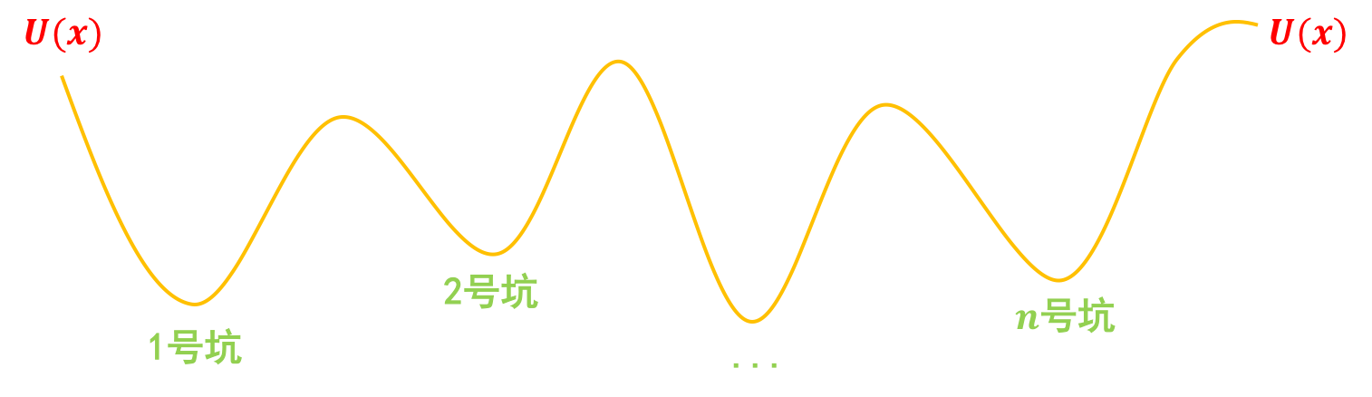GAN step one: "digging pits"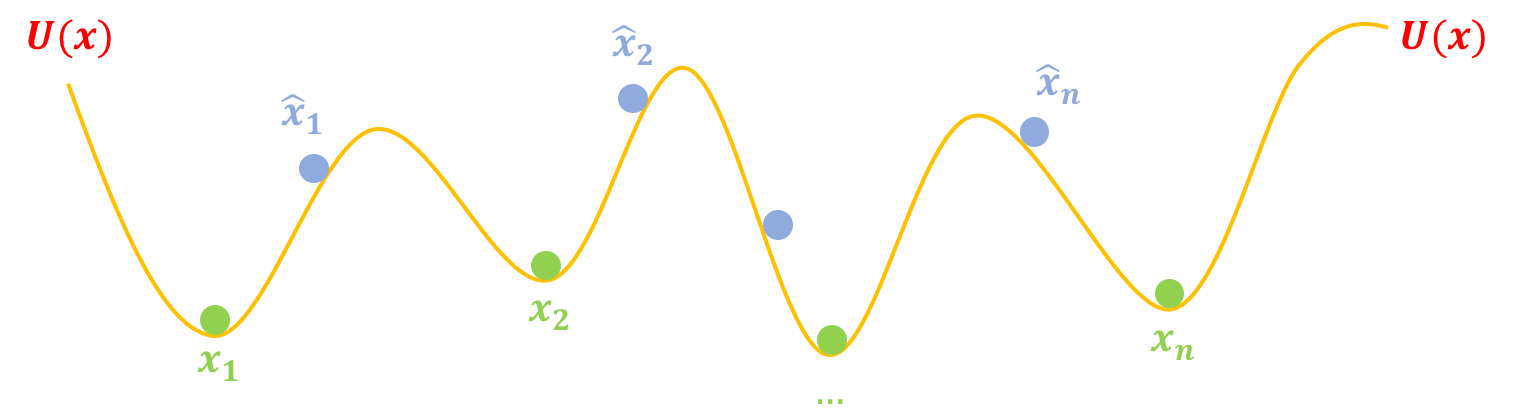Then we place the real and fake samples at their proper positions

"Jumping into Pits"

Step two, jumping into pits: we fix $U(x)$ in place — that is, we stop digging — and then release the fake samples $\hat{x}_1,\hat{x}_2,\dots,\hat{x}_{n}$. Naturally, they gradually roll down to the bottom of the pits, and since the pit bottoms represent the real samples, $\hat{x}_1,\hat{x}_2,\dots,\hat{x}_{n}$ end up looking very much like real samples:

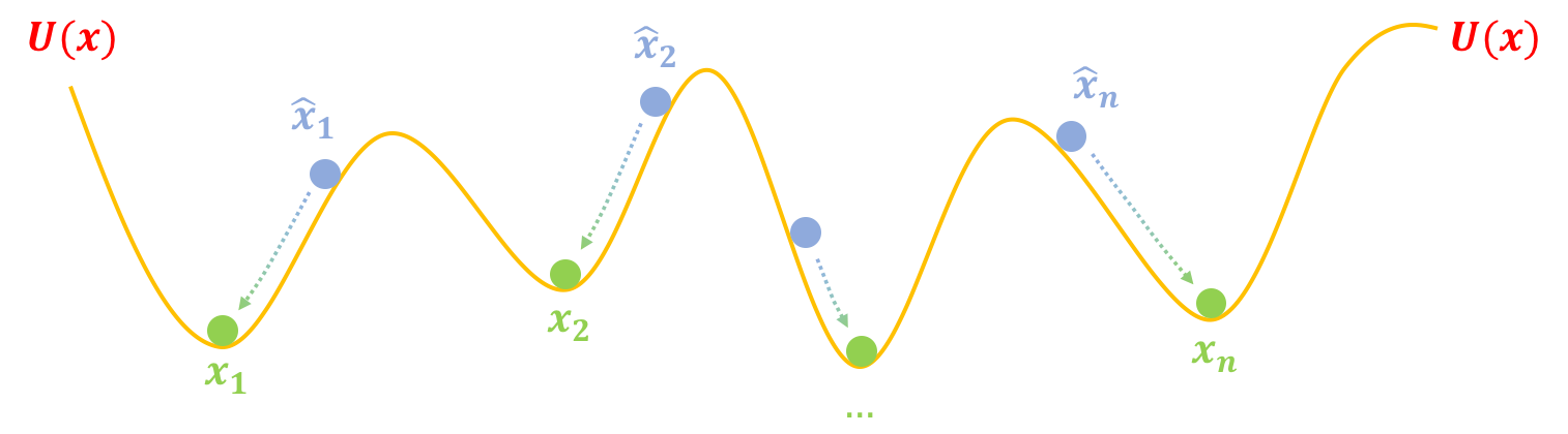GAN step two: "jumping into pits"

That's the whole GAN workflow~

Writing GAN Down

Note that the two steps above aren't just a loose metaphor — they constitute a complete description of GAN. Based on these two steps, we can even write out the GAN training formulas directly.

The Discriminator

Let's first look at "digging pits". We said that real samples should be placed at the bottom of the pits and fake samples on the pit walls, so that the fake samples can later roll down to the bottom. This means the "average altitude" of the fake samples must be higher than the "average altitude" of the real samples, i.e., we want

\begin{equation}\mathbb{E}_{x\sim p(x)}\big[U(x)\big] - \mathbb{E}_{x\sim q(x)}\big[U(x)\big]\label{eq:eq-e}\end{equation}

to be as small as possible, where $p(x)$ denotes the distribution of the real samples and $q(x)$ denotes the distribution of the fake samples. The fake samples are generated via $x=G(z)$, where $z\sim q(z)$ is a standard normal distribution.

Gradient Penalty

Furthermore, we said the real samples should sit at the bottom of the pit. Mathematically, the bottom of a pit is a local minimum, where the derivative should ideally equal 0 — that is, we'd like $\nabla_x U(x)=0$ to hold, or equivalently, as an optimization objective, we want $\Vert \nabla_x U(x)\Vert^2$ to be as small as possible. Combining both requirements gives us the optimization objective for $U$:

\begin{equation}\begin{aligned}U =& \mathop{\text{argmin}}_{U}\mathbb{E}_{x\sim p(x)}\big[U(x)\big] - \mathbb{E}_{x\sim q(x)}\big[U(x)\big] + \lambda \mathbb{E}_{x\sim p(x)}\big[\Vert \nabla_x U(x)\Vert^2\big]\\ =& \mathop{\text{argmin}}_{U}\mathbb{E}_{x\sim p(x)}\big[U(x)\big] - \mathbb{E}_{z\sim q(z)}\big[U(G(z))\big] + \lambda \mathbb{E}_{x\sim p(x)}\big[\Vert \nabla_x U(x)\Vert^2\big] \end{aligned}\label{eq:eq-ee}\end{equation}

Note: In the past, we've always had two points of confusion about gradient penalty: 1) whether the gradient penalty should be centered at 0 or at 1; 2) whether the gradient penalty should be applied to real samples, fake samples, or interpolated real-fake samples. Now, from the energy perspective, we can see that "applying a gradient penalty centered at 0 to the real samples" is the better choice, because this means (on the whole) we want to place the real samples at local minima~
With this, we've arrived at a very intuitive answer to the question of gradient penalty, from the energy point of view.

The Generator

Now let's look at "jumping into pits" — once the pits have been dug and $U$ is fixed, we let the fake samples roll to the bottom of the pits, i.e., we make $U(x)$ decrease, rolling into the nearest pit. So:

\begin{equation}G = \mathop{\text{argmin}}_{G}\mathbb{E}_{z\sim q(z)}\big[U(G(z))\big]\label{eq:eq-g}\end{equation}

As we can see, the discriminator is essentially "shaping the terrain", while the generator is trying to reach the lowest potential energy. This is the core idea of energy-based GANs~

Alternating Training

If the pits in reality were always as simple as in the picture above, then it might only take two steps to fully train a generative model. But in reality the pits can be quite complex — for instance, in the figure below, as the fake sample $\hat{x}_1$ gradually slides down, it might not necessarily reach the pit belonging to $x_1$, but instead land in some intermediate pit. This intermediate pit doesn't represent a real sample — it might just be a "quasi-real" sample. So we need to keep improving the fake samples, and we also need to keep reshaping the pits (for instance, trying to "shave off" the peak that's blocking further progress in the next step). In other words, we need to repeatedly and alternately carry out the two steps $\eqref{eq:eq-e},\eqref{eq:eq-g}$.

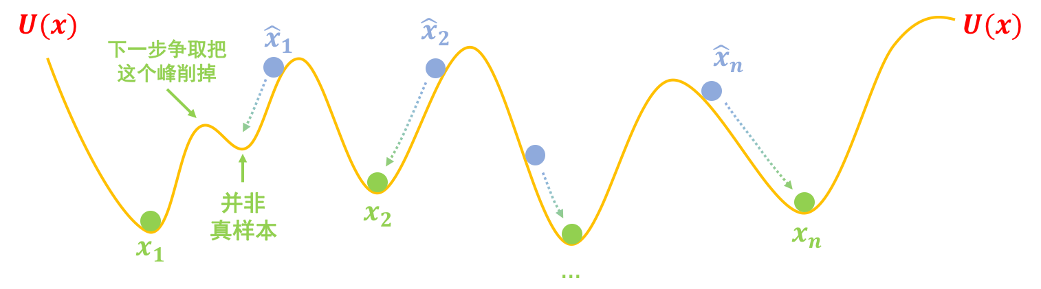In reality, the distribution of pits can be much more complex

The Art of Pits

See — just by imagining a few pits in our minds, we've been able to derive the complete GAN framework, and in fact an upgraded version of the state-of-the-art WGAN-GP: a gradient penalty centered at 0.

GAN is nothing more than the art of digging pits!

For further discussion of this GAN variant, see my earlier blog post WGAN-div: An Unsung Hero That Filled in WGAN's Pits, or the paper Which Training Methods for GANs do actually Converge?.

Further Thoughts

The picture above can also help us answer a lot of questions. For instance, can the discriminator do without gradient penalty? Why is it that most GAN training, especially generator training, avoids momentum-based optimizers — or if a momentum-based optimizer is used, why does the momentum need to be turned down? And how does mode collapse happen?

Hinge Loss

Gradient penalty is theoretically elegant, but it really is quite slow, so from a practical standpoint, it's best to avoid it if possible. But if we skip the gradient penalty and directly minimize equation $\eqref{eq:eq-e}$, we can easily run into numerical instability.

This isn't hard to understand: without any constraint, it's easy to end up with $U(x)\to -\infty$ for real samples and $U(x)\to +\infty$ for fake samples — that is, the discriminator gets optimized too aggressively, pulling the gap too wide (toward infinity). A natural fix is to set a separate threshold for the real and fake samples, so that once the optimization of $U(x)$ passes this threshold, we stop optimizing further. For example:

\begin{equation}\mathbb{E}_{x\sim p(x)}\big[\max(0, 1+U(x))\big] + \mathbb{E}_{x\sim q(x)}\big[\max(0,1-U(x))\big]\label{eq:eq-e-hinge}\end{equation}

This way, for $x\sim p(x)$, if $U(x) < -1$ then $\max(0, 1+U(x))=0$, and for $x\sim q(x)$, if $U(x) > 1$ then $\max(0, 1-U(x))=0$. In both cases we stop optimizing $U(x)$ further — meaning for real samples, $U(x)$ doesn't need to get too small, and for fake samples, $U(x)$ doesn't need to get too large. This prevents $U(x)$ from being over-optimized.

This scheme is exactly the hinge loss used by SNGAN, SAGAN, and BigGAN.

Of course, if $U(x)$ is itself non-negative [for instance, in EBGAN, where the MSE of an autoencoder is used as $U(x)$], then equation $\eqref{eq:eq-e-hinge}$ can be slightly modified to:

\begin{equation}\mathbb{E}_{x\sim p(x)}\big[U(x)\big] + \mathbb{E}_{x\sim q(x)}\big[\max(0,m-U(x))\big]\label{eq:eq-e-hinge2}\end{equation}

where $m > 0$.

Choice of Optimizer

As for the choice of optimizer, we can actually already see the answer from the "jumping into pits" figure.

Momentum-based optimizers help us find better minima faster, but for GANs, we actually don't need to reach a better minimum — we only need to reach the nearest minimum. If we happen to jump out of the nearest minimum and land in a lower one, we might lose diversity, or even trigger mode collapse.

For instance, in the figure below, for the sample $\hat{x}_2$, an optimizer without momentum will let $\hat{x}_2$ roll to $x_2$ and stop there. But with momentum, it might overshoot past $x_2$ and end up all the way at $x_1$. Although $x_1$ is also a real sample, this causes $\hat{x}_1,\hat{x}_2$ to converge toward $x_1$ at the same time as other samples, and perhaps no fake sample is left to generate $x_2$ anymore — thus losing diversity.

Comparison of optimization trajectories with and without momentum: without momentum, fake samples only need to fall into the nearest pit; with momentum, they may overshoot the nearest pit and land in a farther one, causing fake samples to cluster around certain real samples and lose diversity

So, in the optimizer used for GAN training, momentum shouldn't be set too high — too much momentum can actually reduce the diversity of the generated samples, or cause other kinds of instability. Similarly, the learning rate shouldn't be too large either. In short, no acceleration trick should be pushed too hard.

Mode Collapse

What is mode collapse, and why does it happen? Again, this can be easily explained with the same picture.

In the figures drawn earlier, we depicted the fake samples $\hat{x}$ in a reasonably well-spread-out way. But if, due to poor initialization or insufficiently well-behaved optimization, $\hat{x}$ end up clustering around just a few pits, for example:

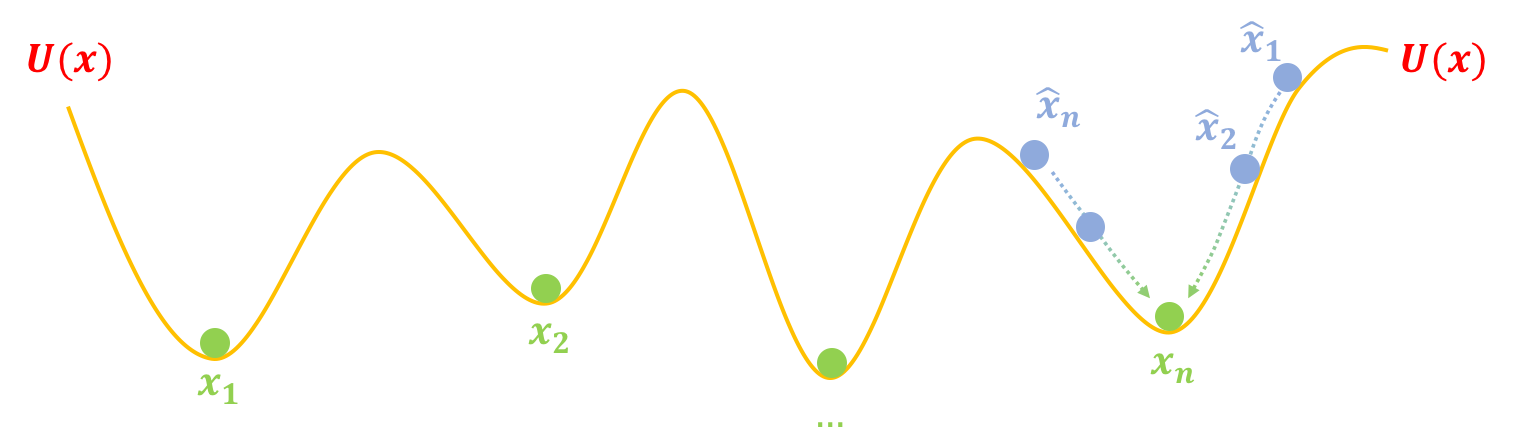Illustration of mode collapse

then, following the optimization process described above, all the fake samples rush toward $x_n$, so the model can only generate samples of a single (or a few) style. This is mode collapse.

Put simply, mode collapse happens because the fake samples are too concentrated, not "uniform" enough. So we can add a term to the generator that encourages the fake samples to spread out more evenly. This term is the entropy $H(X)=H(G(Z))$ of the fake samples — we want this entropy to be as large as possible, meaning more chaotic, more uniform. So the generator's objective can be revised to

\begin{equation}G = \mathop{\text{argmin}}_{G} -H(G(Z)) + \mathbb{E}_{z\sim q(z)}\big[U(G(z))\big]\label{eq:eq-gg}\end{equation}

which, in theory, should solve the mode collapse problem. As for how to compute $H(X)$, we'll get into the details later.

The Beauty of the Energy Perspective

For GANs, the most intuitive and accessible viewpoint is probably the "forger vs. detective" analogy of mutual competition, which directly leads to the standard GAN formulation. But this accessible analogy can't be easily extended to understand WGAN or regularization terms like gradient penalty.

By comparison, the energy perspective is remarkably flexible — it even lets us intuitively understand WGAN, gradient penalty, and other concepts that represent some of the most advanced results in the GAN field today. Although the energy perspective may look formally more complex than the "forger vs. detective" picture, its physical meaning is actually quite clear. With a little thought, we come to find it more interesting and more inspiring — the kind of idea that "grows more flavorful the more you chew on it"~