Unifying Generative Models via Variational Inference (VAE, GAN, AAE, ALI)
Foreword: I've loved pure mathematics since elementary school, and later grew fond of physics too, spending some time studying theoretical physics before gradually moving into machine learning around the time I finished my undergraduate degree. So even within machine learning, my research habits still carry the flavor of mathematics and physics: I try to start from the fewest possible principles and understand — derive — as much as possible from them. This article is one product of that mindset: an attempt to take variational inference as a starting point and use it to give a unified understanding of various models in deep learning, especially the dazzling variety of GANs. This piece has already been posted to arXiv; if you'd like to read the English original, head over to Variational Inference: A Unified Framework of Generative Models and Some Revelations].
Below is the introduction to the article. Actually, the Chinese version may contain slightly more information than the English one — forgive my clumsy English...
Abstract: This paper presents a new perspective on variational inference, showing that the EM algorithm, VAE, GAN, AAE, and ALI (BiGAN) can all be seen as special cases of variational inference. Along the way, the paper also shows that the standard GAN's optimization objective is incomplete, which explains why training GANs requires carefully tuning various hyperparameters. Finally, the paper proposes a regularization term that can remedy this incompleteness, and experiments show that this term improves the stability of GAN training.
In recent years, deep generative models — GANs in particular — have achieved enormous success. By now we can find dozens, if not hundreds, of GAN variants. However, most of these are empirically motivated improvements, with relatively little rigorous theoretical guidance behind them.
The goal of this article is to build a unified framework for these generative models via variational inference. First, I introduce a new formulation of variational inference — one that I've already presented in earlier posts on this blog — which lets us derive the variational autoencoder (VAE) and the EM algorithm in just a few lines. Then, using this same formulation, we can derive GAN directly, and in doing so discover that the standard GAN loss is in fact incomplete: it is missing a regularization term. Without this term, we have to carefully tune the hyperparameters in order to get the model to converge. more
Actually, the original motivation behind this piece of work was simply to bring GAN under the umbrella of variational inference. As it turns out, that original goal has been achieved, and the outcome is quite satisfying. The newly derived regularization term is really a byproduct of this effort — and, fortunately, in our experiments this byproduct actually works.
A New Take on Variational Inference
Suppose $x$ is the observed variable and $z$ is the latent variable, and let $\tilde{p}(x)$ be the evidence distribution of $x$, so that
$$\begin{equation}q(x)=q_{\theta}(x)=\int q_{\theta}(x,z)dz\end{equation}$$
We want $q_{\theta}(x)$ to approximate $\tilde{p}(x)$, so typically we try to maximize the likelihood function
$$\begin{equation}\theta = \mathop{\text{argmax}}_{\theta}\, \int \tilde{p}(x)\log q(x) dx\end{equation}$$
which is equivalent to minimizing the KL divergence $KL(\tilde{p}(x)\Vert q(x))$:
$$\begin{equation}KL(\tilde{p}(x)\Vert q(x)) = \int \tilde{p}(x) \log \frac{\tilde{p}(x)}{q(x)}dx\end{equation}$$
However, since the integral involved may be intractable, direct optimization is difficult in most cases.
In variational inference, we first introduce a joint distribution $p(x,z)$ such that $\tilde{p}(x)=\int p(x,z)dz$, and the essence of variational inference is to replace the KL divergence of the marginal distributions, $KL(\tilde{p}(x)\Vert q(x))$, with the KL divergence of the joint distributions, $KL(p(x,z)\Vert q(x,z))$ or $KL(q(x,z)\Vert p(x,z))$. Since
$$\begin{equation}\begin{aligned}KL(p(x,z)\Vert q(x,z)) &= KL(\tilde{p}(x)\Vert q(x)) + \int \tilde{p}(x) KL(p(z|x)\Vert q(z|x)) dx\\ &\geq KL(\tilde{p}(x)\Vert q(x))\end{aligned}\end{equation}$$
this means that the KL divergence between the joint distributions is a stronger condition (an upper bound). So, once optimization succeeds, we get $q(x,z)\to p(x,z)$, and hence $\int q(x,z)dz \to \int p(x,z)dz = \tilde{p}(x)$, i.e., $\int q(x,z)dz$ becomes an approximation of the true distribution $\tilde{p}(x)$.
Of course, we're not strengthening the condition just for its own sake — we do so because, in many cases, $KL(p(x,z)\Vert q(x,z))$ or $KL(q(x,z)\Vert p(x,z))$ is much easier to compute than $KL(\tilde{p}(x)\Vert q(x))$. So variational inference provides us with a tractable computational scheme.
VAE and the EM Algorithm
From this new understanding of variational inference, we can derive two fundamental results — the variational autoencoder and the EM algorithm — in just a few sentences. This material has actually already been covered in detail in From Maximum Likelihood to the EM Algorithm: A Consistent Perspective] and Variational Autoencoders (II): From a Bayesian Point of View]. Here I'll just restate it briefly.
VAE
In VAE, we set $q(x,z)=q(x|z)q(z), p(x,z)=\tilde{p}(x) p(z|x)$, where $q(x|z),p(z|x)$ is a Gaussian distribution with unknown parameters and $q(z)$ is the standard Gaussian. The objective to be minimized is
$$\begin{equation}\label{eq:kl-oo}KL\left(p(x,z)\Vert q(x,z) \right)=\iint \tilde{p}(x) p(z|x) \log \frac{\tilde{p}(x) p(z|x)}{q(x|z)q(z)}dxdz\end{equation}$$
where $\log \tilde{p}(x)$ doesn't contain the quantity being optimized and can be treated as a constant, while the integral over $\tilde{p}(x)$ is turned into sampling over the data, giving
$$\begin{equation}\mathbb{E}_{x\sim \tilde{p}(x)}\left[-\int p(z|x)\log q(x|z)dz + KL(p(z|x)\Vert q(z))\right]\end{equation}$$
Because $q(x|z),p(z|x)$ is a Gaussian distribution parameterized by a neural network, $KL\left(p(z|x)\Vert q(z)\right)$ can be computed explicitly, and the reparameterization trick lets us sample a point to estimate the integral $\int p(z|x) \log q(x|z)dz$, giving us the final loss that VAE minimizes:
$$\begin{equation}\mathbb{E}_{x\sim \tilde{p}(x)}\Big[-\log q(x|z) + KL(p(z|x)\Vert q(z))\Big]\end{equation}$$
The EM Algorithm
In VAE we constrained the posterior distribution by assuming it is Gaussian, so what we're optimizing are the parameters of that Gaussian. If we drop this assumption and directly optimize the original objective $\eqref{eq:kl-oo}$, this is still workable in some cases, but then we have to resort to alternating optimization: first fix $p(z|x)$ and optimize $q(x|z)$, which gives
$$\begin{equation}\label{eq:em-1}q(x|z) = \mathop{\text{argmax}}_{q(x|z)} \,\mathbb{E}_{x\sim \tilde{p}(x)}\left[\int p(z|x) \log q(x,z) dz\right]\end{equation}$$
Once this step is done, we fix $q(x,z)$ and optimize $p(z|x)$. First rewrite $q(x|z)q(z)$ in the form $q(z|x)q(x)$:
$$\begin{equation}q(x)=\int q(x|z)q(z)dz,\quad q(z|x)=\frac{q(x|z)q(z)}{q(x)}\end{equation}$$
which gives
$$\begin{equation}\begin{aligned}p(z|x) =& \mathop{\text{argmin}}_{p(z|x)} \,\mathbb{E}_{x\sim \tilde{p}(x)}\left[\int p(z|x) \log \frac{p(z|x)}{q(z|x)q(x)} dz\right]\\ =& \mathop{\text{argmin}}_{p(z|x)} \,\mathbb{E}_{x\sim \tilde{p}(x)}\left[KL\left(p(z|x)\Vert q(z|x)\right)-\log q(x)\right]\\ =& \mathop{\text{argmin}}_{p(z|x)} \,\mathbb{E}_{x\sim \tilde{p}(x)} \left[KL\left(p(z|x)\Vert q(z|x)\right)\right] \end{aligned}\end{equation}$$
Since there's now no constraint on $p(z|x)$, we can directly choose $p(z|x)=q(z|x)$ so that the loss equals zero. In other words, $p(z|x)$ has the theoretically optimal solution:
$$\begin{equation}\label{eq:em-2}p(z|x) = \frac{q(x|z)q(z)}{\int q(x|z)q(z)dz}\end{equation}$$
Alternating between these two steps, $\eqref{eq:em-1},\eqref{eq:em-2}$, constitutes the solving procedure of the EM algorithm. In this way, we've quickly recovered the EM algorithm from the variational inference framework.
GAN Under Variational Inference
In this section, we present a general approach for bringing GAN under the umbrella of variational inference, which will lead us to a new understanding of GAN as well as an effective regularization term.
General Framework
Like VAE, GAN also aims to train a generative model $q(x|z)$ that maps $q(z)=N(z;0,I)$ to the data distribution $\tilde{p}(x)$. But unlike VAE, which chooses $q(x|z)$ to be Gaussian, GAN chooses
$$\begin{equation}q(x|z)=\delta\left(x - G(z)\right),\quad q(x)=\int q(x|z)q(z)dz\end{equation}$$
where $\delta(x)$ is the Dirac $\delta$ function and $G(z)$ is the generator's neural network.
We would normally think of $z$ as a latent variable, but since the $\delta$ function actually represents a point mass distribution, the relationship between $x$ and $z$ is already one-to-one — so the relationship between $z$ and $x$ is "not random enough." In GAN, we therefore don't treat it as a latent variable (meaning we don't need to consider the posterior $p(z|x)$).
In fact, in GAN we only introduce a binary latent variable $y$ to form the joint distribution
$$\begin{equation}q(x,y)=\left\{\begin{aligned}&\tilde{p}(x)p_1,\,y=1\\&q(x)p_0,\,y=0\end{aligned}\right.\end{equation}$$
Here $p_1 = 1-p_0$ describes a two-point distribution, and we simply take $p_1=p_0=1/2$. On the other hand, we set $p(x,y)=p(y|x) \tilde{p}(x)$, where $p(y|x)$ is a conditional Bernoulli distribution. The optimization objective is the reverse-direction $KL\left(q(x,y)\Vert p(x,y) \right)$:
$$\begin{equation}\begin{aligned}KL\left(q(x,y)\Vert p(x,y) \right)=&\int \tilde{p}(x)p_1\log \frac{\tilde{p}(x)p_1}{p(1|x)\tilde{p}(x)}dx+\int q(x)p_0\log \frac{q(x)p_0}{p(0|x)\tilde{p}(x)}dx\\ \sim&\int \tilde{p}(x)\log \frac{1}{p(1|x)}dx+\int q(x)\log \frac{q(x)}{p(0|x)\tilde{p}(x)}dx\end{aligned}\end{equation}$$
Once optimization succeeds, we get $q(x,y)\to p(x,y)$, and hence
$$\begin{equation}p_1 \tilde{p}(x) + p_0 q(x) = \sum_y q(x,y) \to \sum_y p(x,y) = \tilde{p}(x)\end{equation}$$
so that $q(x)\to\tilde{p}(x)$, which completes the construction of the generative model.
Now the objects we're optimizing are $p(y|x)$ and $G(x)$; write $p(1|x)=D(x)$, which is the discriminator. Just like with the EM algorithm, we perform alternating optimization: first fix $G(z)$ (which also fixes $q(x)$), and then optimize $p(y|x)$. Dropping the constants, the optimization objective becomes:
$$\begin{equation}D = \mathop{\text{argmin}}_{D} -\mathbb{E}_{x\sim\tilde{p}(x)}\left[\log D(x)\right]-\mathbb{E}_{x\sim q(x)}\left[\log (1-D(x))\right]\end{equation}$$
Then we fix $D(x)$ and optimize $G(x)$, for which the relevant loss is:
$$\begin{equation}\label{eq:gan-g-loss}G = \mathop{\text{argmin}}_{G}\int q(x)\log \frac{q(x)}{(1-D(x)) \tilde{p}(x)}dx\end{equation}$$
This involves the unknown $\tilde{p}(x)$, but if the $D(x)$ model has sufficient fitting capacity, then, by the same reasoning as in equation $\eqref{eq:em-2}$, the optimal solution for $D(x)$ should be
$$\begin{equation}D(x)=\frac{\tilde{p}(x)}{\tilde{p}(x)+q^{o}(x)}\end{equation}$$
where $q^{o}(x)$ here denotes the $q(x)$ from the previous step. Solving this for $\tilde{p}(x)$ and substituting into $\eqref{eq:gan-g-loss}$ gives
$$\begin{equation}\begin{aligned}\int q(x)\log \frac{q(x)}{D(x) q^{o}(x)}dx=&-\mathbb{E}_{x\sim q(x)}\log D(x) + KL\left(q(x)\Vert q^{o}(x)\right)\\ =&-\mathbb{E}_{z\sim q(z)}\log D(G(z)) + KL\left(q(x)\Vert q^{o}(x)\right) \end{aligned}\end{equation}$$
Basic Analysis
As we can see, the first term is one of the standard losses used for the GAN generator.
$$\begin{equation}-\mathbb{E}_{z\sim q(z)}\log D(G(z))\end{equation}$$
The extra second term describes the distance between the new and old distributions. These two loss terms are in tension with each other: $KL\left(q(x)\Vert q^{o}(x)\right)$ wants the new and old distributions to be as close as possible, but if the discriminator has been sufficiently optimized, then for samples drawn from the old distribution $q^{o}(x)$, $D(x)$ will be small (since they're almost all classified as negative samples), which makes $-\log D(x)$ fairly large, and vice versa. As a result, when we optimize the whole loss jointly, the model both has to "inherit" the old distribution $q^{o}(x)$ and, at the same time, explore in the direction of the new distribution $p(1|y)$ — interpolating between old and new.
We know that the current standard GAN generator loss doesn't include $KL\left(q(x)\Vert q^{o}(x)\right)$ at all, which is exactly what makes the loss incomplete. Suppose there existed an optimization algorithm that always found the theoretically optimal solution for $G(z)$, and that $G(z)$ had unlimited fitting capacity — then $G(z)$ would only need to generate a single sample that maximizes $D(x)$ (regardless of the input $z$), which is exactly mode collapse. Put this way, it would in fact be theoretically inevitable.
So, what insight does $KL\left(q(x)\Vert q^{o}(x)\right)$ give us? Let's write
$$\begin{equation}q^{o}(x)=q_{\theta-\Delta \theta}(x),\quad q(x)=q_{\theta}(x)\end{equation}$$
That is, suppose the current model's parameters change by an amount $\Delta\theta$. Expanding to second order, we get
$$\begin{equation}KL\left(q(x)\Vert q^{o}(x)\right)\approx \int\frac{\left(\Delta\theta\cdot \nabla_{\theta}q_{\theta}(x)\right)^2}{2q_{\theta}(x)} dx \approx \left(\Delta\theta\cdot c\right)^2\end{equation}$$
We've already pointed out that a complete GAN generator loss should include $KL\left(q(x)\Vert q^{o}(x)\right)$. If it doesn't, we have to achieve the same effect through various indirect means, and the approximation above shows that the extra loss incurred is roughly $\left(\Delta\theta\cdot c\right)^2$, which means we must keep it from becoming too large — that is, we must keep $\Delta\theta$ from getting too large (at each stage, $c$ can be treated approximately as a constant). Since we're using gradient-descent-based optimization, $\Delta\theta$ is proportional to the gradient, which explains many of the tricks commonly used in GAN training — gradient clipping, using the Adam optimizer, using batch normalization — all of these serve to stabilize the gradient so that $\theta$ doesn't get too large. At the same time, the number of iterations for $G(z)$ shouldn't be too high either, since too many iterations will likewise cause $\Delta\theta$ to grow too large.
Also, this analysis applies only to the generator — the discriminator itself is unconstrained, so the discriminator can be trained to optimality.
The Regularization Term
Now let's extract something genuinely useful from this: we directly estimate $KL\left(q(x)\Vert q^{o}(x)\right)$ to obtain a regularization term we can actually use in practice. Direct computation is intractable, but we can approximate it using $KL\left(q(x,z)\Vert \tilde{q}(x,z)\right)$:
$$\begin{equation}\begin{aligned}KL\left(q(x,z)\Vert \tilde{q}(x,z)\right)=&\iint q(x|z)q(z)\log \frac{q(x|z)q(z)}{\tilde{q}(x|z)q(z)}dxdz\\ =&\iint \delta\left(x-G(z)\right)q(z)\log \frac{\delta\left(x-G(z)\right)}{\delta\left(x-G^{o}(z)\right)}dxdz\\ =&\int q(z)\log \frac{\delta(0)}{\delta\left(G(z)-G^{o}(z)\right)}dz \end{aligned}\end{equation}$$
Since there's a limit
$$\begin{equation}\delta(x)=\lim_{\sigma\to 0}\frac{1}{(2\pi\sigma^2)^{d/2}}\exp\left(-\frac{x^2}{2\sigma^2}\right)\end{equation}$$
we can treat $\delta(x)$ as a low-variance Gaussian distribution, and substituting gives us
$$\begin{equation}KL\left(q(x)\Vert q^{o}(x)\right)\sim \lambda \int q(z)\Vert G(z) - G^{o}(z)\Vert^2 dz\end{equation}$$
So the loss of the complete generator can be chosen as
$$\begin{equation}\mathbb{E}_{z\sim q(z)}\left[-\log D(G(z))+\lambda \Vert G(z) - G^{o}(z)\Vert^2\right] \end{equation}$$
That is, we can use the distance between newly and previously generated samples as a regularization term, which ensures the model doesn't stray too far from the old distribution.
The two experiments below on the CelebA face dataset show that this regularization term does indeed help. The experimental code is modified from here] and is currently hosted on my GitHub].
Experiment 1: A standard DCGAN network, where each iteration trains one batch each for generator and discriminator.
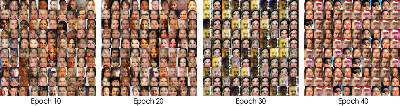 ] Without the regularization term, the model starts to collapse after 25 epochs
 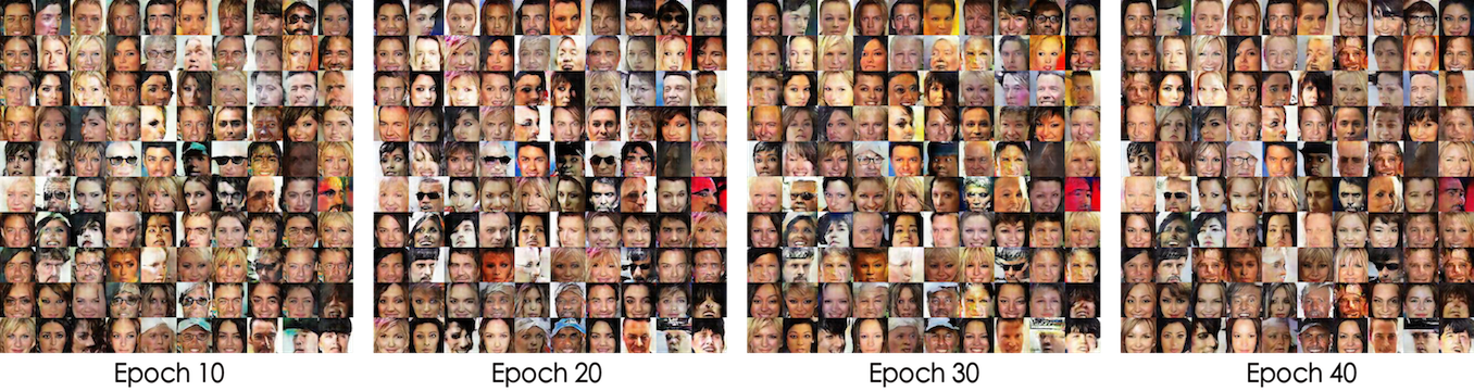 ] With the regularization term, the model trains stably throughout
Experiment 2: A standard DCGAN network with BN removed, where each iteration trains five batches each for generator and discriminator.
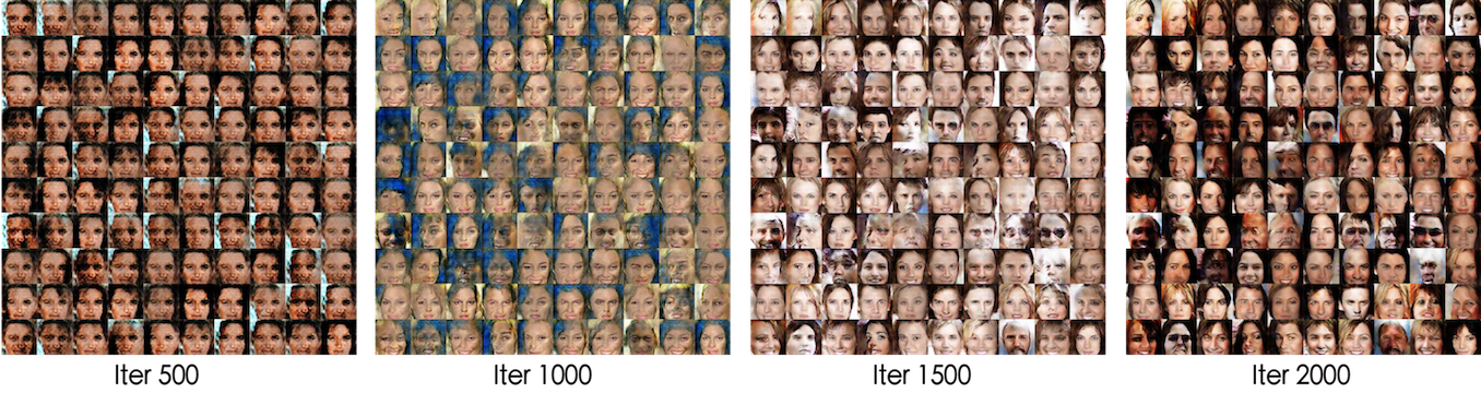 ] Without the regularization term, the model converges relatively slowly
 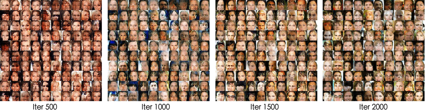 ] With the regularization term, the model "gets on track" faster
GAN-Related Models
Adversarial Autoencoders (AAE) and Adversarially Learned Inference (ALI, closely related to Bidirectional GAN) are both GAN variants, and they too can be brought under the variational inference umbrella. Given all the groundwork above, deriving them is really just like solving two homework problems.
Interestingly, ALI leads us to some counterintuitive results.
AAE from a GAN Perspective
It turns out that simply swapping the roles of $x,z$ in the GAN derivation gives us the AAE framework.
Specifically, AAE aims to train an encoder model $p(z|x)$ that maps the true distribution $\tilde{q}(x)$ to the standard Gaussian $q(z)=N(z;0,I)$, where
$$\begin{equation}p(z|x)=\delta\left(z - E(x)\right),\quad p(z)=\int p(z|x)\tilde{q}(x)dx\end{equation}$$
and $E(x)$ is the encoder's neural network.
Just as with GAN, AAE introduces a binary latent variable $y$, giving
$$\begin{equation}p(z,y)=\left\{\begin{aligned}&p(z)p_1,\,y=1\\&q(z)p_0,\,y=0\end{aligned}\right.\end{equation}$$
and again we simply take $p_1=p_0=1/2$. On the other hand, we set $q(z,y)=q(y|z) q(z)$, where the posterior $p(y|z)$ is a binary distribution taking $z$ as input, and then optimize $KL\left(p(z,y)\Vert q(z,y) \right)$:
$$\begin{equation}\begin{aligned}KL\left(p(z,y)\Vert q(z,y) \right)=&\int p(z)p_1\log \frac{p(z)p_1}{q(1|z)q(z)}dz+\int q(z)p_0\log \frac{q(z)p_0}{q(0|z)q(z)}dz\\ \sim&\int p(z)\log \frac{p(z)}{q(1|z)q(z)}dz+\int q(z)\log \frac{1}{q(0|z)}dz\end{aligned}\end{equation}$$
Now the objects we're optimizing are $q(y|z)$ and $E(x)$; write $q(0|z)=D(z)$. Again we alternate: first fix $E(x)$ (which also fixes $p(z)$), and then optimize $q(y|z)$. Dropping the constants, the optimization objective is:
$$\begin{equation}\begin{aligned}D=\mathop{\text{argmin}}_D &-\mathbb{E}_{z\sim p(z)}\left[\log (1-D(z))\right]-\mathbb{E}_{z\sim q(z)}\left[\log D(z)\right]\\ =\mathop{\text{argmin}}_D &-\mathbb{E}_{z\sim \tilde{p}(x)}\left[\log (1-D(E(x)))\right]-\mathbb{E}_{z\sim q(z)}\left[\log D(z)\right]\end{aligned}\end{equation}$$
Then fix $D(z)$ and optimize $E(x)$, for which the relevant loss is:
$$\begin{equation}E = \mathop{\text{argmin}}_E \int p(z)\log \frac{p(z) }{(1-D(z)) q(z)}dz\end{equation}$$
Using the theoretically optimal solution $D(z)=q(z)/[p^{o}(z)+q(z)]$ for $D(z)$ and substituting into the loss gives
$$\begin{equation}\mathbb{E}_{x\sim \tilde{p}(x)}[-\log D(E(x))] + KL\left(p(z)\Vert p^{o}(z)\right)\end{equation}$$
On the one hand, just as with standard GAN, careful training allows us to drop the second term, giving
$$\begin{equation}\mathbb{E}_{x\sim \tilde{p}(x)}[-\log D(E(x))]\end{equation}$$
On the other hand, we can obtain an encoder and then separately train a decoder $G(z)$; but if the assumed fitting capacity of $E(x),G(z)$ is sufficient that the reconstruction error can be made small enough, then adding $G(z)$ to the loss above won't interfere with GAN training, so we can train them jointly:
$$\begin{equation}G,E = \mathop{\text{argmin}}_{G,E}\mathbb{E}_{x\sim \tilde{p}(x)}\left[-\log D(E(x))+\lambda\Vert x - G(E(x))\Vert^2\right]\end{equation}$$
A Counterintuitive Version of ALI
ALI is like a fusion of GAN and AAE; another almost identical piece of work is Bidirectional GAN (BiGAN). Compared to GAN, it also brings $z$ into the variational inference framework as a latent variable. Specifically, in ALI we have
$$\begin{equation}q(x,z,y)=\left\{\begin{aligned}&p(z|x)\tilde{p}(x) p_1,\,y=1\\&q(x|z)q(z)p_0,\,y=0\end{aligned}\right.\end{equation}$$
as well as $p(x,z,y)=p(y|x,z) p(z|x) \tilde{p}(x)$, and we then optimize $KL\left(q(x,z,y)\Vert p(x,z,y) \right)$:
$$\begin{equation}\begin{aligned}&\iint p(z|x)\tilde{p}(x) p_1\log \frac{p(z|x)\tilde{p}(x) p_1}{p(1|x,z) p(z|x) \tilde{p}(x)}dxdz\\ +&\iint q(x|z)q(z)p_0\log \frac{q(x|z)q(z)p_0}{p(0|x,z) p(z|x) \tilde{p}(x)}dxdz\end{aligned}\end{equation}$$
which is equivalent to minimizing
$$\begin{equation}\label{eq: ori-loss-ali}\iint p(z|x)\tilde{p}(x)\log \frac{1}{p(1|x,z)}dxdz+\iint q(x|z)q(z)\log \frac{q(x|z)q(z)}{p(0|x,z) p(z|x) \tilde{p}(x)}dxdz\end{equation}$$
Now the objects being optimized are $p(y|x,z),p(z|x),q(x|z)$; write $p(1|x,z)=D(x,z)$, where $p(z|x)$ is a Gaussian or Dirac distribution parameterized by encoder $E$, and $q(x|z)$ is a Gaussian or Dirac distribution parameterized by generator $G$. Again we alternate optimization: first fix $E,G$, so that the loss relevant to $D$ is
$$\begin{equation}D=\mathop{\text{argmin}}_D -\mathbb{E}_{x\sim\tilde{p}(x),z\sim p(z|x)} \log D(x,z) - \mathbb{E}_{z\sim q(z),x\sim q(x|z)} \log (1-D(x,z))\end{equation}$$
Just as with VAE, the expectations over $p(z|x)$ and $q(x|z)$ can be handled via the reparameterization trick. Next we fix $D$ and optimize $G,E$. Since we now have both $E$ and $G$, the whole loss can't be simplified further and still looks like $\eqref{eq: ori-loss-ali}$. But using the optimal solution for $D$,
$$\begin{equation}D(x,z)=\frac{p^{o}(z|x)\tilde{p}(x)}{p^{o}(z|x)\tilde{p}(x)+q^{o}(x|z)q(z)}\end{equation}$$
it can be transformed into
$$\begin{equation}\begin{aligned}-\iint p(z|x)\tilde{p}(x)\log D(x, z) dxdz -\iint q(x|z) q(z)\log D(x, z) dxdz\\ +\int q(z) KL(q(x|z)\Vert q^o(x|z)) dz + \iint q(x|z) q(z)\log \frac{p^o(z|x)}{p(z|x)}dxdz\end{aligned}\end{equation}$$
Since $q(x|z),p(x|z)$ are all Gaussian distributions, we can in fact compute the last two terms explicitly (with the help of the reparameterization trick), but just as with standard GAN, careful training allows us to simply drop these two terms, giving
$$\begin{equation}\label{eq:our-ali-g}-\iint p(z|x)\tilde{p}(x)\log D(x, z) dxdz -\iint q(x|z) q(z)\log D(x, z) dxdz\end{equation}$$
This is the generator and encoder loss for ALI that we've derived, and it differs from the standard ALI result. Standard ALI (including plain GAN) treats the problem as a minimax problem, so the generator and encoder loss is
$$\begin{equation}\label{eq:our-ali-g-o1}\iint p(z|x)\tilde{p}(x)\log D(x, z) dxdz + \iint q(x|z) q(z)\log (1-D(x, z)) dxdz\end{equation}$$
or
$$\begin{equation}\label{eq:our-ali-g-o2}-\iint p(z|x)\tilde{p}(x)\log (1-D(x, z)) dxdz -\iint q(x|z) q(z)\log D(x, z) dxdz\end{equation}$$
Neither of these is equivalent to $\eqref{eq:our-ali-g}$. Regarding this discrepancy, I did in fact run experiments, and the results show that this version of ALI performs just as well as the standard version — possibly even slightly better (though that might just be my own wishful bias, so I won't include the figures). This suggests that treating an adversarial network as a minimax problem is merely an intuitive convention, not something that must necessarily be the case.
Concluding Remarks
The results in this article show that variational inference really is a unified framework for deriving and explaining generative models, including both VAE and GAN. Through this new interpretation of variational inference, we've shown how it achieves this goal.
Of course, this article isn't the first to propose using variational inference to study GANs. In On Unifying Deep Generative Models], the authors also attempt to unify VAE and GAN using variational inference, and they too obtain some illuminating results. But I feel that paper isn't as clear as it could be. In fact, I never fully understood it — I'm not entirely sure whether it brings GAN under the umbrella of variational inference, or whether it instead folds VAE into GAN. By comparison, I think the exposition in this article is clearer and more definite.
It seems there's still a lot of room left to explore in variational inference, waiting for us to dig into.
Translated automatically with claude-sonnet-5; all equations are reproduced verbatim from the source. Copyright remains with the original author.