O-GAN: A Simple Modification That Turns a GAN Discriminator into an Encoder!

O-GAN：简单修改，让GAN的判别器变成一个编码器！ 苏剑林 · 2019-03-06 · Machine Learning unsupervised GAN generative model encoding

In this post I want to share a recent piece of work of mine: by making a simple modification to the standard GAN model, we can turn the discriminator into an encoder, so that a GAN simultaneously has both generative and encoding capability — with almost no extra training cost. This new model is called O-GAN (Orthogonal GAN, i.e. Orthogonal Generative Adversarial Network), because it is built around an orthogonal decomposition operation applied to the discriminator, which is the fullest possible exploitation of the discriminator's degrees of freedom.

Arxiv link: https://papers.cool/arxiv/1903.01931
Open-source code: https://github.com/bojone/o-gan

Background

I've been deep in the rabbit hole of generative models for quite a while now. Not only have I written a number of blog posts on generative models, I've also submitted several small papers on the topic to arxiv. Over the course of falling deeper into this hole, my understanding of generative models — GANs in particular — has gradually deepened, and at times I've felt I'd made some improvement worth writing up (that's why I submitted them to arxiv). But truthfully, most of that work was minor patchwork of little real consequence.

The model I'm introducing in this post, I dare say, is worth more than the sum total of all my previous GAN-related work: it offers what is currently the simplest scheme for training a GAN model that has encoding capability.

By now GANs have become quite mature, and models keep getting bigger and bigger — the likes of BigGAN and StyleGAN, generally recognized as the most advanced GANs around, are already well known and widely played with. However, these state-of-the-art GAN models currently only have a generator function, not an encoder function: they can produce an endless stream of new images, but they cannot extract features from existing images.

Of course, there has been plenty of research on GANs equipped with encoders — even this blog has covered one (see BiGAN-QP: A Simple and Clear Encoding & Generative Model). But whether or not a GAN has encoding capability, most GANs share one feature: once training is finished, the discriminator becomes useless. In theory, the more it's trained, the more the discriminator degenerates (e.g. it tends toward a constant).

Anyone who has trained a GAN knows that the discriminator and generator networks are of comparable complexity (and if there's an encoder too, it's comparable in complexity as well). Throwing away the discriminator once GAN training is done is really a severe waste of this large network! Generally speaking, the discriminator's architecture is quite similar to that of an encoder, so a natural idea is: can we make the discriminator and the encoder share most of their weights? As far as I know, among all previous GAN-related models, only IntroVAE managed to achieve this. But IntroVAE's approach is comparatively complicated, and there's still no successful open-source reproduction of IntroVAE online (I tried to reproduce it myself, and failed too).

The scheme in this post, by contrast, is extremely simple — by slightly modifying the original GAN model, we can turn the discriminator into an encoder, with virtually no increase in either complexity or computational cost.

The Model

Without further ado, let's introduce this model. First, let's write down a general form of GAN:

\begin{equation}\begin{aligned}D =& \mathop{\text{argmin}}_{D} \mathbb{E}_{x\sim p(x), z\sim q(z)}\Big[f(D(x)) + g(D(G(z)))\Big]\\ G =& \mathop{\text{argmin}}_{G} \mathbb{E}_{z\sim q(z)}\Big[h(D(G(z)))\Big] \end{aligned}\end{equation}

To avoid confusion, let me painstakingly clarify the notation. Here $x\in \mathbb{R}^{n_x},z\in \mathbb{R}^{n_z}$, $p(x)$ is the "evidence distribution" of the real image set, and $q(z)$ is the noise distribution (in this post it is a $n_z$-dimensional standard normal distribution); $G: \mathbb{R}^{n_z} \to \mathbb{R}^{n_x}$ and $D: \mathbb{R}^{n_x} \to \mathbb{R}$ are, naturally, the generator and discriminator, and $f,g,h$ are certain fixed functions — different GANs correspond to different choices of $f,h,g$. Sometimes we add normalization or regularization tricks such as spectral normalization or gradient penalty; for simplicity these will not be written out explicitly.

Next, let's define a few vector operators:

\begin{equation}\text{avg}(z)=\frac{1}{n_z}\sum_{i=1}^{n_z} z_i,\quad \text{std}(z)=\sqrt{\frac{1}{n_z}\sum_{i=1}^{n_z} (z_i-\text{avg}(z))^2}, \quad \mathcal{N}(z)=\frac{z - \text{avg}(z)}{\text{std}(z)}\end{equation}

This looks rather fancy written out, but it's really just the mean and variance of the elements of a vector, and the standardized (normalized) vector. In particular, when $n_z \geq 3$ (which is satisfied by all genuinely useful GANs), $\left[\text{avg}(z), \text{std}(z), \mathcal{N}(z)\right]$ is independent of the mean and variance — that is, it corresponds to an "orthogonal decomposition" of the original vector $z$.

Next, we've already said that the discriminator's structure is somewhat similar to that of an encoder, except that the encoder outputs a vector while the discriminator outputs a scalar. So we can write the discriminator as a composite function:

\begin{equation}D(x)\triangleq T(E(x))\end{equation}

Here $E$ is a mapping $\mathbb{R}^{n_x} \to \mathbb{R}^{n_z}$, and $T$ is a mapping $\mathbb{R}^{n_z} \to \mathbb{R}$. It's not hard to imagine that $E$ has far more parameters than $T$, so we would like $E(x)$ to have encoding capability.

How do we achieve this? We simply add a loss: the Pearson correlation coefficient!

\begin{equation}\begin{aligned}T,E =& \mathop{\text{argmin}}_{T,E} \mathbb{E}_{x\sim p(x), z\sim q(z)}\Big[f(T(E(x))) + g(T(E(G(z)))) - \lambda \rho(z, E(G(z)))\Big]\\ G =& \mathop{\text{argmin}}_{G} \mathbb{E}_{z\sim q(z)}\Big[h(T(E(G(z)))) - \lambda \rho(z, E(G(z)))\Big] \end{aligned}\end{equation}

where

\begin{equation}\rho(z, \hat{z})=\frac{\sum\limits_{i=1}^{n_z} (z_i - \text{avg}(z))(\hat{z}_i - \text{avg}(\hat{z}))/n_z}{\text{std}(z)\times \text{std}(\hat{z})}=\cos(\mathcal{N}(z), \mathcal{N}(E(G(z))))\end{equation}

If $\lambda=0$, then this is just a plain GAN (only, the discriminator has been split into two parts, $E$ and $T$). Once we add this correlation term, intuitively speaking, we're asking that $z$ and $E(G(z))$ be as linearly correlated as possible. Why does this work? We'll leave the discussion of that until the end.

Clearly this correlation coefficient can be plugged into essentially any existing GAN, and the amount of code change is small (split the discriminator into two parts, add one loss term). I've run experiments on several different GANs and found that training succeeds in every case.

With this, the GAN's discriminator $D$ is split into two parts, $E$ and $T$, and $E$ becomes an encoder — meaning that most of the discriminator's parameters are now put to use. But $T$ still remains, and after training $T$ is also useless. Although $T$ has relatively few parameters, so the waste is small, for someone with "OCD tendencies" (like me), this is still uncomfortable.

Can we also get rid of $T$? After many rounds of experimentation, the conclusion is: yes, we really can! Because we can directly use $\text{avg}(E(x))$ as the discriminator:

\begin{equation}\begin{aligned}E =& \mathop{\text{argmin}}_{E} \mathbb{E}_{x\sim p(x), z\sim q(z)}\Big[f(\text{avg}(E(x))) + g(\text{avg}(E(G(z)))) - \lambda \rho(z, E(G(z)))\Big]\\ G =& \mathop{\text{argmin}}_{G} \mathbb{E}_{z\sim q(z)}\Big[h(\text{avg}(E(G(z)))) - \lambda \rho(z, E(G(z)))\Big] \end{aligned}\label{eq:simplest}\end{equation}

With this, there's no longer any $T$ in the whole model at all — only the pure generator $G$ and the encoder $E$, with not a shred of redundancy left anywhere in the model (fellow OCD sufferers can now rest easy).

Experiments

Why does this work? We'll leave that discussion till the end. Let's first look at the experimental results — after all, no matter how elegant the theory sounds, it means nothing if the experiments don't hold up.

Note that, in theory, the correlation term introduced in this post shouldn't improve the quality of the generative model per se; so the experiments have two main goals: 1) does this extra loss harm the quality of the original generative model; 2) does this extra loss really turn $E$ into an effective encoder?

As mentioned, this method can be plugged into any GAN. In this experiment I use a variant of my earlier GAN-QP:

\begin{equation}\begin{aligned}E =& \mathop{\text{argmin}}_{E} \mathbb{E}_{x\sim p(x), z\sim q(z)}\Big[\text{avg}(E(x)) - \text{avg}(E(G(z))) + \lambda_1 R_{x,z} - \lambda_2 \rho(z, E(G(z)))\Big]\\ G =& \mathop{\text{argmin}}_{G} \mathbb{E}_{z\sim q(z)}\Big[\text{avg}(E(G(z))) - \lambda_2 \rho(z, E(G(z)))\Big] \end{aligned}\label{eq:simplest-2}\end{equation}

where

\begin{equation}R_{x,z} = \frac{[\text{avg}(E(x)) - \text{avg}(E(G(z)))]^2}{\Vert x - G(z)\Vert^2}\end{equation}

For the datasets, this round of experiments is fairly comprehensive — I ran experiments on CelebA HQ, FFHQ, LSUN-church outdoor, and LSUN-bedroom, all at a resolution of $128\times 128$ (I also did a bit of experimentation at $256\times 256$, with decent results too, but that didn't make it into the paper). The model architecture is DCGAN as usual; for the rest of the details, please refer directly to the paper or the code.

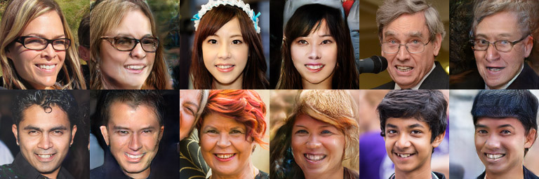
Images above:

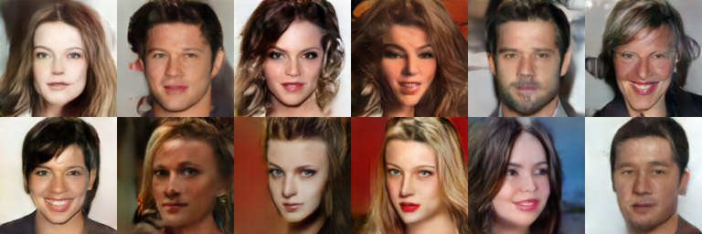CelebA HQ random generation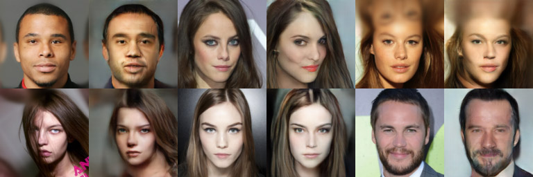CelebA HQ reconstruction results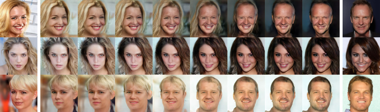CelebA HQ linear interpolation

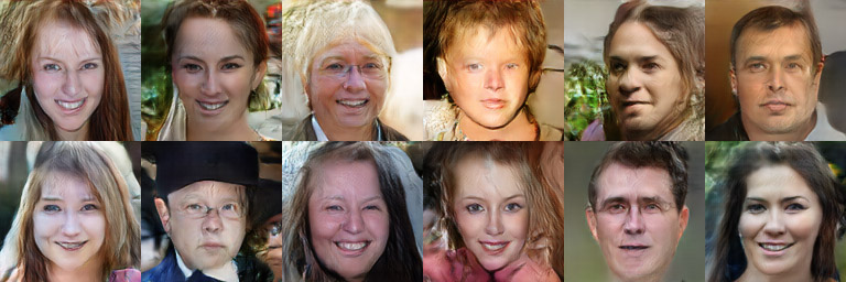FFHQ random generationFFHQ reconstruction results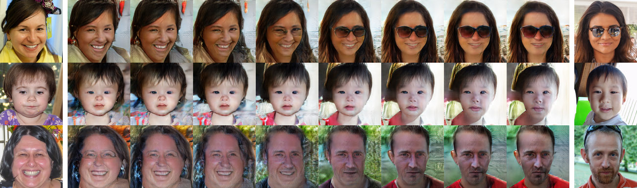FFHQ linear interpolation

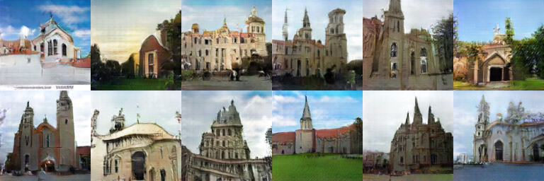LSUN-church random generationLSUN-church reconstruction results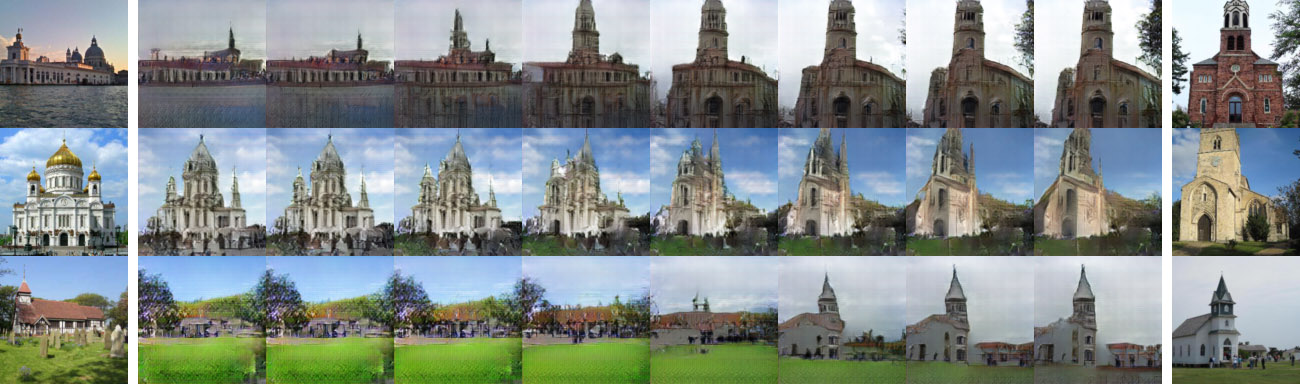LSUN-church linear interpolation

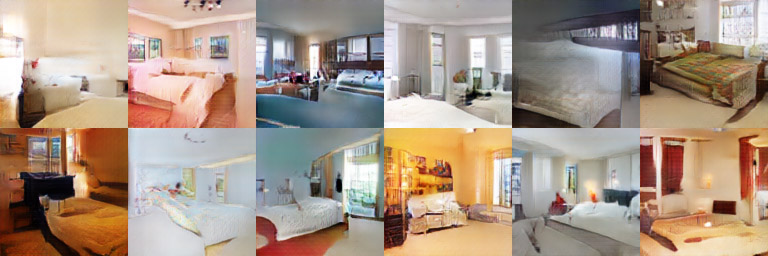LSUN-bedroom random generationLSUN-bedroom reconstruction results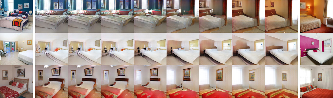LSUN-bedroom linear interpolation

Whether or not you find these convincing, I personally think they look pretty good~

1. Random generation results are decent, showing that the newly introduced correlation term doesn't degrade generation quality;
2. Reconstruction results are decent, showing that $E(x)$ has indeed captured the main features of $x$;
3. Linear interpolation results are decent, showing that $E(x)$ has indeed learned features that are close to linearly separable.

The Underlying Principle

OK, now that we've confirmed — via a look in the eye, or rather, a look at the results — that it works, let's discuss why.

Clearly, the role of this extra reconstruction term is to make $z$ as "correlated" with $E(G(z))$ as possible. For this, most readers' first instinct would probably be the MSE loss $\Vert z - E(G(z))\Vert^2$ rather than the $\rho(z, E(G(z)))$ used here. But in fact, if we use $\Vert z - E(G(z))\Vert^2$, training basically always fails. So why does $\rho(z, E(G(z)))$ succeed?

By the earlier definitions, $E(x)$ outputs a $n_z$-dimensional vector, but $T(E(x))$ outputs only a scalar — that is, $E(x)$ has $n_z$ degrees of freedom, while the discriminator $T(E(x))$ needs to occupy at least one degree of freedom (in principle it only needs exactly one). If we minimize $\Vert z - E(G(z))\Vert^2$, the training process forces $E(G(z))$ to become exactly equal to $z$, meaning all $n_z$ degrees of freedom get taken up by it, leaving none for the discriminator to use for telling real from fake — which is why adding $\Vert z - E(G(z))\Vert^2$ is very likely to fail. But $\rho(z, E(G(z)))$ is different: $\rho(z, E(G(z)))$ has nothing to do with $\text{avg}(E(G(z)))$ or $\text{std}(E(G(z)))$ (it only changes the $E(G(z))$ and $\text{avg}$ of the vector $\text{std}$, without changing the value of $\rho(z, E(G(z)))$, because $\rho$ itself has already had its mean subtracted and been divided by its standard deviation). This means that even if we maximize $\rho(z, E(G(z)))$, we still leave at least two degrees of freedom for the discriminator.

This is also why in $\eqref{eq:simplest}$ we can even directly use $\text{avg}(E(x))$ as the discriminator, since it's unaffected by $\rho(z, E(G(z)))$.

A similar example is InfoGAN. InfoGAN also includes a module that reconstructs part of the input information, a module which also shares most of its weights with the discriminator (the encoder). Because InfoGAN in fact only reconstructs part of the input information, the reconstruction term doesn't use up all the degrees of freedom of the encoder — so InfoGAN's approach is reasonable, as long as at least one degree of freedom is left for the discriminator.

There's another fact that can help us understand this. During adversarial training, the noise is $z\sim \mathcal{N}(0,I_{n_z})$-distributed; once the generator is well trained, then in theory, for any $z\sim \mathcal{N}(0,I_{n_z})$, $G(z)$ should be a realistic image. In fact, the converse also holds: if $G(z)$ is a realistic image, then we should have $z\sim \mathcal{N}(0,I_{n_z})$ (i.e. it lies in a region of high probability under $\mathcal{N}(0,I_{n_z})$). Carrying this reasoning further, for $z\sim \mathcal{N}(0,I_{n_z})$, we have $\text{avg}(z)\approx 0$ as well as $\text{std}(z)\approx 1$. So, if $G(z)$ is a realistic image, then a necessary condition is $\text{avg}(z)\approx 0$ together with $\text{std}(z)\approx 1$.

Applying this conclusion: if we want good reconstruction quality, i.e. we want $G(E(x))$ to be a realistic image, then a necessary condition is $\text{avg}(E(x))\approx 0$ together with $\text{std}(E(x))\approx 1$. This tells us that for a good $E(x)$, we can treat $\text{avg}(E(x))$ and $\text{std}(E(x))$ as already known (equal to 0 and 1, respectively). Since they're already known, there's no need to fit them — in other words, we can exclude them from the reconstruction term. And indeed:

\begin{equation}-\rho(z, E(G(z)))\sim \left\Vert \mathcal{N}(z) - \mathcal{N}(E(G(z)))\right\Vert^2\end{equation}

That is, if we exclude $\text{avg}(E(x))$ and $\text{std}(E(x))$ from the MSE loss and drop the constant, it reduces exactly to $-\rho(z, E(G(z)))$, which again confirms the reasonableness of $\rho(z, E(G(z)))$. Furthermore, this derivation shows that the reconstruction process is not $G(E(x))$ but rather

\begin{equation}\hat{x}=G(\mathcal{N}(E(x)))\end{equation}

Finally, in theory this extra reconstruction term should also help prevent mode collapse. This is fairly intuitive — since reconstruction quality is already good, the generation quality can't be too bad either, so naturally there's not much room for mode collapse. If a more mathematical justification is wanted, we can interpret $\rho(z, E(G(z)))$ as a lower bound on the mutual information between $Z$ and $G(Z)$, so minimizing $-\rho(z, E(G(z)))$ is effectively maximizing the mutual information between $Z$ and $G(Z)$, which in turn is equivalent to maximizing the entropy of $G(Z)$. And when the entropy of $G(Z)$ increases, that indicates greater diversity, which moves it further away from mode collapse. For a similar line of reasoning, see An Energy Perspective on GANs (II): GAN = "Analysis" + "Sampling".

Conclusion

This post has introduced a scheme that, through a simple modification of the original GAN, turns the GAN's discriminator into an effective encoder. Multiple experiments show that this scheme works, and further reflection on the underlying principle reveals that it is essentially an orthogonal decomposition of the original discriminator (encoder), together with a full exploitation of the resulting degrees of freedom — hence the name "Orthogonal GAN (O-GAN)".

A small modification that nets you an encoder for free — why not? Everyone is welcome to give it a try~

Afterword:
Looking back, the idea behind this model is essentially a decomposition into "magnitude and direction," which isn't hard to understand in retrospect — but actually arriving at it wasn't easy at all.
At first I kept getting stuck in the trap of $\Vert z - E(G(z))\Vert^2$, unable to break free. Later I tried various tricks and eventually managed to stabilize the model (after months of effort) using a reconstruction loss based on $\Vert z - E(G(z))\Vert^2$, but the resulting model was quite ugly (it introduced a triple-adversarial GAN), so I set about simplifying it. Later I tried using the $\cos$ value with a reconstruction loss, and found, surprisingly, that it converged easily — which got me thinking about the underlying reason, and it probably comes down to degrees of freedom.
Next I tried decomposing $E(x)$ into a magnitude and a direction vector, then used the magnitude $\Vert E(x)\Vert$ as the discriminator and $\cos$ for the reconstruction loss, with a hinge loss for the discriminator. This has a fairly clear geometric meaning, and sounds nicer in principle; it worked on some datasets (CelebA was fine, but LSUN wasn't), and there was another problem: $\Vert E(x)\Vert$ is non-negative, so it can't be plugged into a general GAN, and many of the standard tricks for stabilizing GAN training couldn't be used.
Then I thought about how to make the magnitude able to take both positive and negative values. I started by considering taking the log of the magnitude, so that magnitudes below 1 become negative after the log and magnitudes above 1 become positive — which achieves the desired effect. Unfortunately, the results still weren't good. After a series of further unsuccessful experiments, I finally realized I could give up on the magnitude (which corresponds to variance) as the discriminator's loss, and just use the mean directly instead~ So eventually it turned into $\text{avg}(E(x))$ — this transition took quite a long time.
Also, reconstruction loss is normally thought to need to measure the difference between $x$ and $G(E(x))$, but I found that it's enough to measure the difference between $z$ and $E(G(z))$ — this is the lowest-cost option, since reconstruction requires extra time anyway. Finally, I ran a great many other experiments; many ideas that succeeded on CelebA simply didn't work on LSUN. So while the final model looks simple, it's really the product of a long, hard process of distillation.
The whole model grew out of one fixation of mine: given that the discriminator has the structure of an encoder, it shouldn't be wasted. Combined with the prior success of IntroVAE, I was convinced there must be a simpler way to achieve this. After months of experiments, running upwards of a hundred models, I finally managed to fully solve this problem just recently.
Oh, and besides IntroVAE, another paper that inspired me a great deal is Deep Infomax — its appendix offers a new way of thinking about how to build a GAN, and that's actually where I started when thinking through this new model.