BiGAN-QP: A Simple and Clean Encoding & Generative Model

BiGAN-QP：简单清晰的编码&生成模型 苏剑林 · 2018-12-10 · Machine Learning unsupervised GAN generative model encoding

Not long ago, by working directly in the dual space, I proposed an adversarial modeling framework called GAN-QP, whose distinguishing feature is that it can be proven theoretically to avoid both vanishing gradients and the need for a Lipschitz constraint, which greatly simplifies the construction and training of generative models.

GAN-QP is an adversarial framework, so in principle all of the usual GAN tasks can be tried with it. In the earlier post A GAN Without the L Constraint and Without Vanishing Gradients?], we only tried the standard random generation task. In this post, we try a setting that has both a generator and an encoder: BiGAN-QP.

BiGAN and BiGAN-QP

Note that this is BiGAN, not the BigGAN that was so popular a while back. BiGAN stands for Bidirectional GAN, proposed in the paper Adversarial Feature Learning]. Around the same time there was a very similar paper called Adversarially Learned Inference], which proposed a model called ALI, quite similar to BiGAN. Broadly speaking, both of these add an encoder into the ordinary GAN setup, so that the model retains the random-generation ability of a normal GAN while also gaining the ability to extract useful features via the encoder. Applying the GAN-QP adversarial scheme to BiGAN gives us BiGAN-QP.

Without further ado, here are some example results (left is the original image, right is the reconstruction):

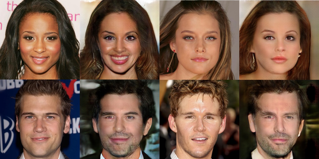BiGAN-QP reconstruction example]

more

This was obtained by reducing 256×256×3 images down to 256 dimensions and then reconstructing them. As you can see, the overall reconstruction quality is quite good, without the blurriness typical of ordinary autoencoders. Some details are missing—compared to IntroVAE] it's a bit weaker—but that's a matter of model architecture and hyperparameter tuning, which isn't really my area of expertise. Regardless, these results should be enough to show that BiGAN-QP works, and works reasonably well.

The content of this post has already been incorporated into the original GAN-QP paper: https://papers.cool/arxiv/1811.07296], and readers can download the latest version from arxiv.

A Concise Derivation of BiGAN-QP

Compared to GAN, the derivation of BiGAN is actually very simple—you just need to replace the original single input $x$ with the paired input $(x,z)$. Likewise, once you have the foundation of GAN-QP, the so-called BiGAN-QP is also very straightforward. Specifically, the original GAN-QP looked like this:

\begin{equation}\begin{aligned}&T= \mathop{\text{argmax}}_T\, \mathbb{E}_{(x_r,x_f)\sim p(x_r)q(x_f)}\left[T(x_r,x_f)-T(x_f,x_r) - \frac{(T(x_r,x_f)-T(x_f,x_r))^2}{2\lambda d(x_r,x_f)}\right] \\ &G = \mathop{\text{argmin}}_G\,\mathbb{E}_{(x_r,x_f)\sim p(x_r)q(x_f)}\left[T(x_r,x_f)-T(x_f,x_r)\right] \end{aligned}\end{equation}

and now it becomes:

\begin{equation}\begin{aligned}T&= \mathop{\text{argmax}}_T\, \mathbb{E}_{x\sim p(x), z\sim q(z)}\left[\Delta T - \frac{\Delta T^2}{2\lambda d\big(x,E(x);G(z),z\big)}\right] \\ G,E &= \mathop{\text{argmin}}_{G,E}\,\mathbb{E}_{x\sim p(x), z\sim q(z)}[\Delta T]\\ \Delta T &= T(x,E(x);G(z),z)-T(G(z),z;x,E(x)) \end{aligned}\end{equation}

or, in the simplified version, we just take $\Delta T = T(x,E(x))-T(G(z),z)$ directly. In principle, that's all there is to it—this is BiGAN-QP.

In practice, however, it's hard to learn a good bidirectional mapping this way, because it amounts to automatically searching for one particular bidirectional mapping out of countless possible ones, which is a fairly difficult task. So we still need some "guiding terms." We use two mse losses as guiding terms:

\begin{equation}\begin{aligned}T&= \mathop{\text{argmax}}_T\, \mathbb{E}_{x\sim p(x), z\sim q(z)}\left[\Delta T - \frac{\Delta T^2}{2\lambda d\big(x,E(x);G(z),z\big)}\right] \\ G,E &= \mathop{\text{argmin}}_{G,E}\,\mathbb{E}_{x\sim p(x), z\sim q(z)}\Big[\Delta T + \beta_1 \Vert z - E(G(z))\Vert^2 + \beta_2 \Vert x - G(E(x))\Vert^2\Big]\\ \Delta T &= T(x,E(x))-T(G(z),z) \end{aligned}\end{equation}

Each of the three loss terms for the generator is fairly intuitive: $\Delta T$ pushes the generated images to be more realistic, $\Vert z - E(G(z))\Vert^2$ aims to reconstruct the latent variable space, and $\Vert x - G(E(x))\Vert^2$ aims to reconstruct the observed variable space. The latter two terms shouldn't be too large—especially the last one, since making it too large leads to blurry images.

These two regularization terms can be viewed as upper bounds on the mutual information between $G(z)$ and $z$, and between $x$ and $E(x)$, respectively. So from an information-theoretic perspective, these two regularization terms are trying to make the mutual information between $x,z$ as large as possible. For related discussion, see the InfoGAN] paper—these two regularization terms mean that our model also belongs to the InfoGAN family. So, strictly speaking, this should really be called Bi-Info-GAN-QP.
The mutual information terms can, to some extent, stabilize the GAN training process and reduce the likelihood of mode collapse, since once mode collapse occurs, the mutual information can no longer stay large. In other words, if the model collapses, reconstruction becomes essentially impossible, and the reconstruction loss will blow up.

Experiments show that with a small additional adjustment, the results get even better. This adjustment comes from the observation that the two mse terms, when coupled together, are still too powerful (the loss value itself may not be large, but the gradients are), which still tends to make the model produce blurry images. So we need to stop half of the gradient flow, giving:

\begin{equation}\begin{aligned}T&= \mathop{\text{argmax}}_T\, \mathbb{E}_{x\sim p(x), z\sim q(z)}\left[\Delta T - \frac{\Delta T^2}{2\lambda d\big(x,E(x);G(z),z\big)}\right] \\ G,E &= \mathop{\text{argmin}}_{G,E}\,\mathbb{E}_{x\sim p(x), z\sim q(z)}\Big[\Delta T + \beta_1 \Vert z - E(G_{ng}(z))\Vert^2 + \beta_2 \Vert x - G(E_{ng}(x))\Vert^2\Big]\\ \Delta T &= T(x,E(x))-T(G(z),z) \end{aligned}\end{equation}

$G_{ng}$ and $E_{ng}$ mean forcibly setting the gradient of that part to zero; most frameworks provide this operator directly, so you can just call it. This is the final form of the BiGAN-QP model presented in this post.

Code and Results

The code has also been added to Github: https://github.com/bojone/gan-qp/tree/master/bigan-qp]

Here are some more results, this time from random generation:

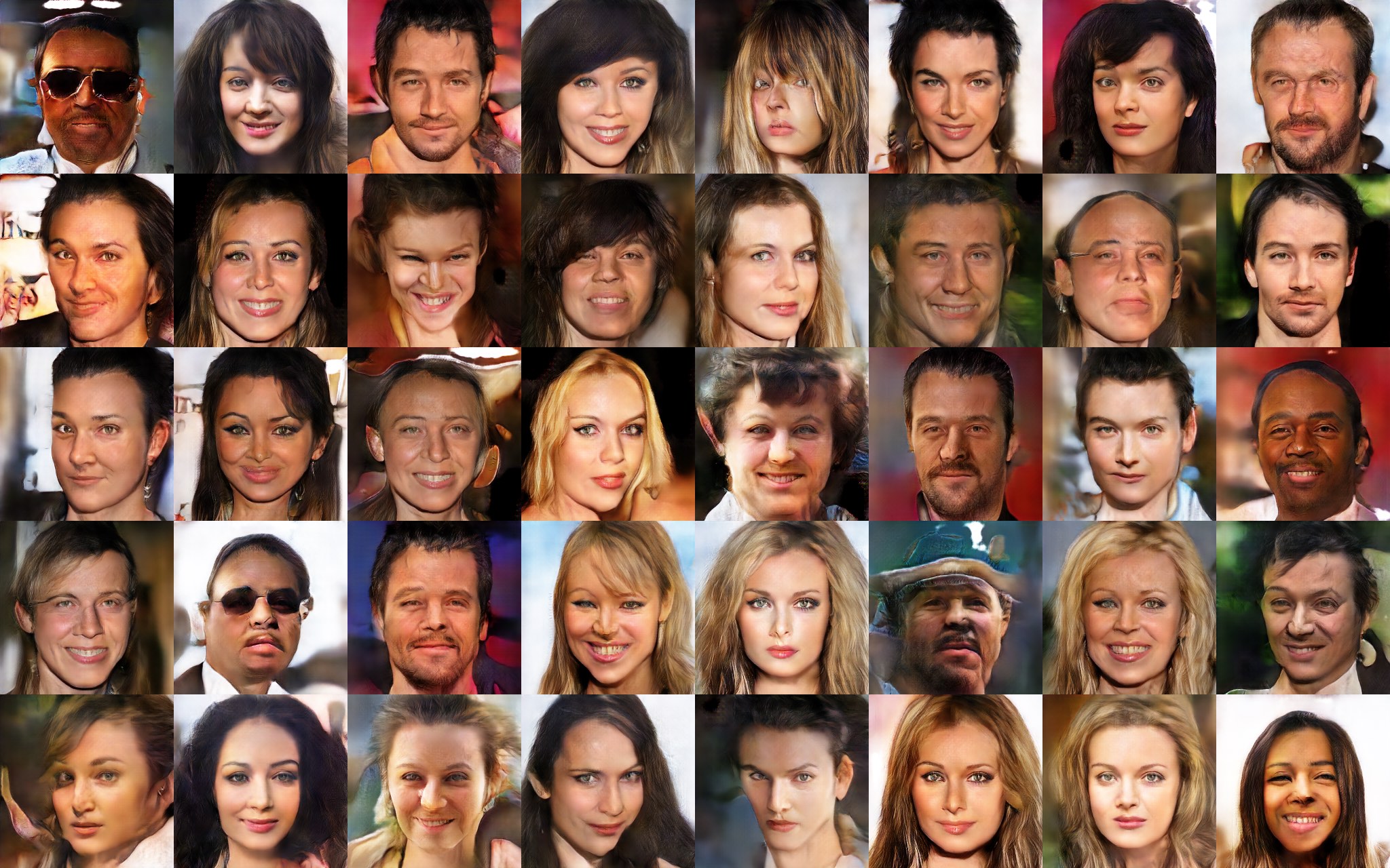BiGAN-QP randomly generated images]

Reconstructions (left is original, right is reconstruction):

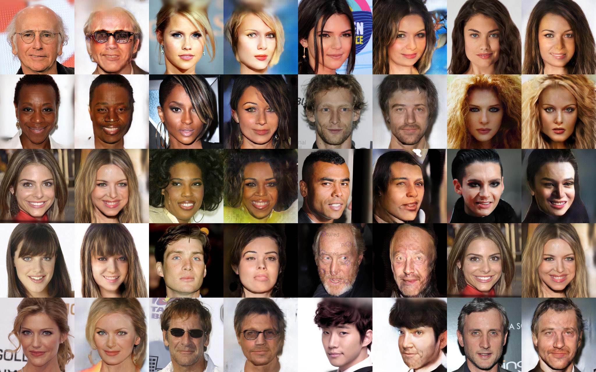BiGAN-QP reconstruction example 2]

As you can see, whether it's random generation or reconstruction, the results are satisfying, with no sign of blurriness—showing that we have indeed successfully trained a GAN model that has both encoding and generation capabilities.

An important feature to note here is that, because this is dimensionality-reduced reconstruction, the model does not (and cannot) learn a pixel-perfect one-to-one mapping. Instead, it produces a reconstruction that looks overall similar and is nonetheless sharp. For example, look at the first image in the first row and the second image in the last row: the model has basically reconstructed the person, but interestingly, with the glasses—we can see that the model does reconstruct glasses, but of a different "style." We could even say that the model has learned the concept of "glasses"; it's just that, due to dimensionality reduction, the latent representation's capacity is limited, so although the model knows there are glasses there, it can't reproduce the exact same pair, and instead substitutes a common alternative style.

This is something that ordinary VAEs, which demand "point-by-point one-to-one reconstruction," cannot achieve—and that very requirement of point-by-point correspondence is also the main reason VAEs produce blurry results. If you want fully invertible reconstruction, only an invertible model like Glow] can achieve that.

Also, since we have both an encoder and a generator, we can play around with latent-space interpolation between real images:

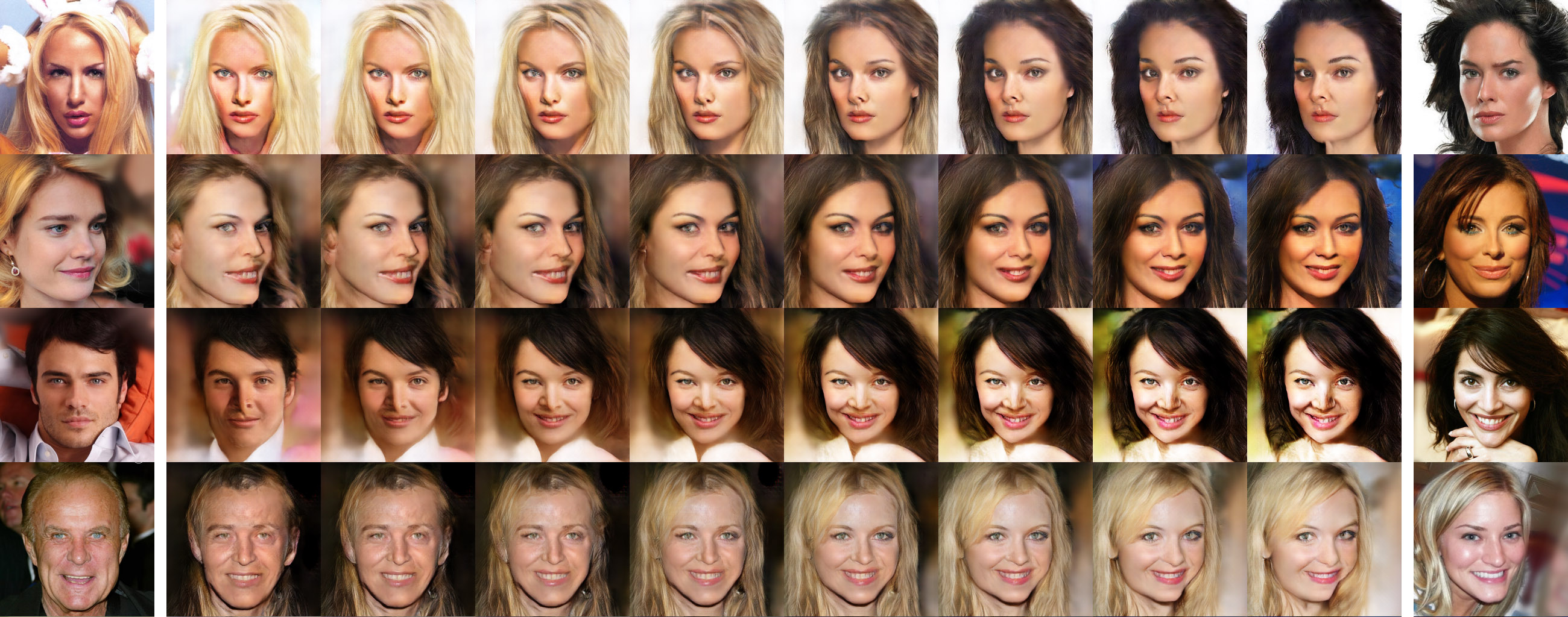BiGAN-QP interpolation between real images (the leftmost and rightmost are real images, the second-from-left and second-from-right are their reconstructions, and the rest are interpolations)]

We can also look at what BiGAN-QP considers to be "similar" images (compute the latent variables of all real images, then measure similarity via Euclidean distance or cosine similarity, and find the most similar ones; the figure below shows the Euclidean distance results):

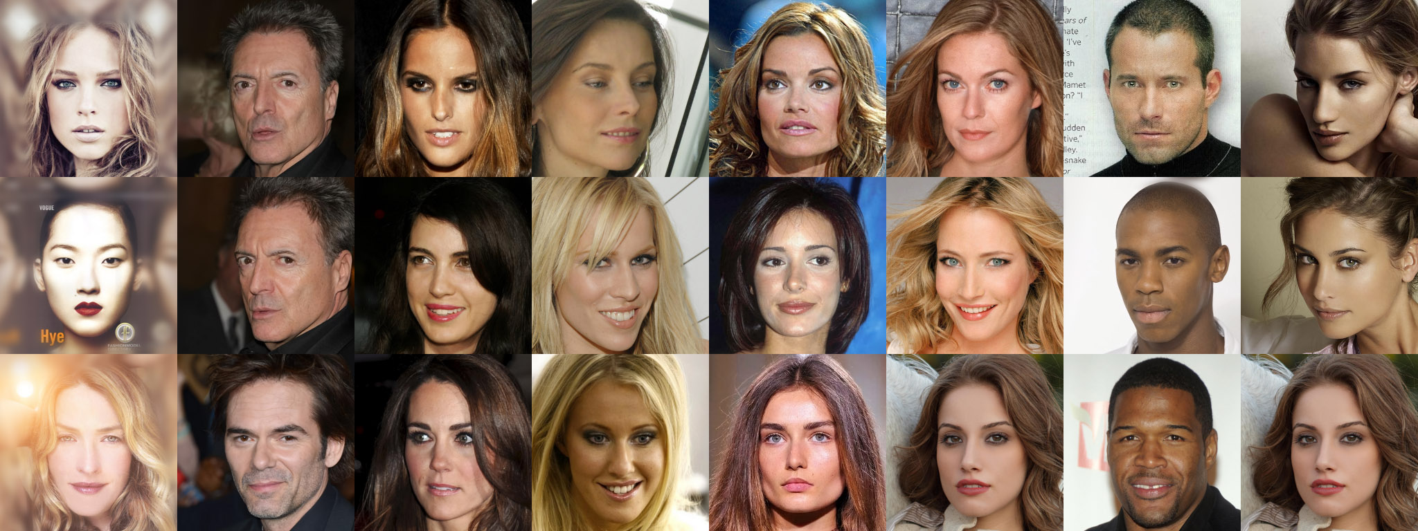Similar images as seen by BiGAN-QP (the first row is the input, the following two rows are the similar images)]

Feel Free to Use and Share

As mentioned above, GAN-QP is a theoretically complete adversarial framework, and in principle all sorts of GAN tasks can be tried with it. So if you happen to have a GAN task at hand, why not give it a try? You'll be able to drop the Lipschitz constraint, drop spectral normalization, and even drop many of the regularization terms, all without having to worry about vanishing gradients. GAN-QP is the result of my ongoing effort to strip away the various hyperparameters that plague GANs.

If you have new application results based on GAN-QP, feel free to share them here.