Mutual Information in Deep Learning: Unsupervised Feature Extraction

深度学习的互信息：无监督提取特征 苏剑林 · 2018-10-02 · Machine Learning maximum entropy unsupervised mutual information

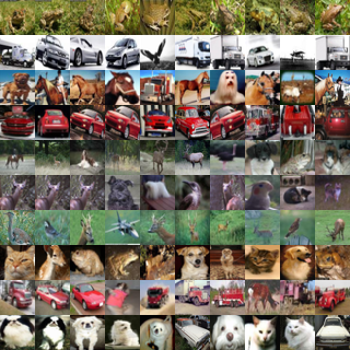Randomly sampled KNN examples

For NLP, mutual information is a very important metric that measures the intrinsic relatedness between two things. I have discussed mutual information many times on this blog, and I'm generally quite interested in papers that make use of mutual information. A few days ago I came across the recently proposed Deep INFOMAX model on Jiqizhixin, which uses mutual information maximization to perform unsupervised learning on images. Naturally I found it quite interesting, studied it carefully, and this post is the result.

The overall approach here follows the original Deep INFOMAX paper, but I haven't simply copied the original model — I've modified it according to my own ideas (mainly the part about the prior distribution), and I'll point this out at the relevant places.

What Are We Trying to Do

Autoencoders

Feature extraction is an important and fundamental task in unsupervised learning; a common approach is to train an encoder that maps raw data into a fixed-length vector. Naturally, our basic requirement for this encoder is: it should preserve (as much as possible of) the important information in the original data.

How do we know that the encoded vector preserves the important information? A natural idea is that the encoded vector should also be able to reconstruct the original image, so we also train a decoder that tries to reconstruct the original image, with the final loss being the MSE between the original and reconstructed images. This leads to the design of the standard autoencoder. Later, we also wanted the distribution of the encoded vectors to be as close as possible to a Gaussian distribution, which leads to the variational autoencoder (VAE).

Rethinking Reconstruction

However, it's worth thinking about whether this "reconstruction" requirement is actually reasonable.

First, we can observe that reconstructions of the original image from a low-dimensional code tend to be quite blurry. This can be explained by the fact that the MSE loss requires "pixel-by-pixel" reconstruction, which is a very harsh requirement. Or we could understand it this way: for image reconstruction, we don't actually have a particularly suitable loss to use — the ideal approach would be to use an adversarial network to train a discriminator, but that further increases the difficulty of the task.

Second, here's an interesting fact: most of us can distinguish a lot of real bills from fake ones, but if you asked us to draw a hundred-dollar bill from memory, I'm confident the result would look nothing like the real thing. This shows that, for a task like counterfeit detection, we can imagine having a pile of real and fake bills to learn from — we can extract very rich features from them, but these features aren't sufficient to reconstruct the original image; they only let us tell the bills apart. In other words, for a given dataset and task, reasonable, sufficient features don't necessarily allow image reconstruction.

Maximizing Mutual Information

Mutual Information

The discussion above shows that reconstruction is not a necessary condition for good features. The basic principle of a good feature should be "being able to distinguish this sample from the entire dataset" — that is, extracting the (most) unique information about that sample. How do we measure whether the extracted information is unique to the sample? We use "mutual information" to measure this.

Let's introduce some notation: let $X$ denote the set of original images, $x\in X$ a particular original image, $Z$ the set of encoded vectors, $z\in Z$ a particular encoded vector, and $p(z|x)$ the distribution of the encoded vector produced by $x$ — we take this to be a Gaussian distribution, or simply think of it as the encoder we're trying to find. Then we can use mutual information to express the relatedness of $X,Z$:

$$\begin{equation}I(X,Z) = \iint p(z|x)\tilde{p}(x)\log \frac{p(z|x)}{p(z)}dxdz\label{eq:mi}\end{equation}$$

Here $\tilde{p}(x)$ is the distribution of the original data, and $p(z)$ is the distribution over the whole of $Z$ given a fixed $p(z|x)$, i.e.

$$\begin{equation}p(z) = \int p(z|x)\tilde{p}(x)dx\end{equation}$$

Then a good feature encoder should make the mutual information as large as possible, i.e.

$$\begin{equation}p(z|x) = \mathop{\text{argmax}}_{p(z|x)} I(X,Z) \end{equation}$$

A larger mutual information means that (most of) $\log \frac{p(z|x)}{p(z)}$ should be as large as possible, which means $p(z|x)$ should be much larger than $p(z)$ — that is, for each $x$, the encoder should be able to find the $z$ specific to $x$, such that the probability of $p(z|x)$ is much larger than the random probability $p(z)$. In this way, we gain the ability to identify the original sample purely from $z$.

Note: the quantity $\eqref{eq:mi}$ is called mutual information, while the log term $\log \frac{p(z|x)}{p(z)}$ is called "pointwise mutual information," though it's sometimes also just called mutual information. The difference between the two: $\eqref{eq:mi}$ measures an overall relationship, e.g. answering the question "are the two words in front of and after each other related at all?"; $\log \frac{p(z|x)}{p(z)}$ measures a local relationship, e.g. answering "do '忐' and '忑' frequently appear together?"

Prior Distribution

As mentioned earlier, compared to a plain autoencoder, a VAE additionally wants the latent variable to follow a standard normal prior distribution, which helps make the encoding space more regular and may even help disentangle features, facilitating downstream learning. So here we'd also like to add this constraint.

The Deep INFOMAX paper introduces this constraint through an AAE-like adversarial approach, but as is well known, adversarial training is a min-max process requiring alternating optimization, which is neither very stable nor very simple. Here I offer a more end-to-end alternative: let $q(z)$ be the standard normal distribution, and let's minimize the KL divergence between $p(z)$ and the prior $q(z)$:

$$\begin{equation}\label{eq:prior}KL(p(z)\Vert q(z))=\int p(z)\log \frac{p(z)}{q(z)}dz\end{equation}$$

Combining $\eqref{eq:mi}$ and $\eqref{eq:prior}$ with weights, we get the overall objective to minimize:

$$\begin{equation}\begin{aligned}p(z|x) =& \min_{p(z|x)} \left\{- I(X,Z) + \lambda KL(p(z)\Vert q(z))\right\}\\ =&\min_{p(z|x)}\left\{-\iint p(z|x)\tilde{p}(x)\log \frac{p(z|x)}{p(z)}dxdz + \lambda\int p(z)\log \frac{p(z)}{q(z)}dz\right\}\end{aligned}\label{eq:total-loss-1}\end{equation}$$

This looks clean and nice, but we still don't know the expression for $p(z)$, so we can't actually compute anything yet — this story isn't over.

Solving It Piece by Piece

Simplifying the Prior Term

Interestingly, if we rearrange the loss in equation $\eqref{eq:total-loss-1}$ a bit, we get:

$$\begin{equation}p(z|x) =\min_{p(z|x)}\left\{\iint p(z|x)\tilde{p}(x)\left[-(1+\lambda)\log \frac{p(z|x)}{p(z)} + \lambda \log \frac{p(z|x)}{q(z)}\right]dxdz\right\}\end{equation}$$

Notice that the expression above is exactly a weighted sum of the mutual information and $\mathbb{E}_{x\sim\tilde{p}(x)}[KL(p(z|x)\Vert q(z))]$, and the term $KL(p(z|x)\Vert q(z))$ is something we can compute directly (it's exactly the KL divergence term from VAE). So we've already solved half of the total loss, which we can write as

$$\begin{equation}p(z|x) =\min_{p(z|x)}\left\{-\beta\cdot I(X,Z)+\gamma\cdot \mathbb{E}_{x\sim\tilde{p}(x)}[KL(p(z|x)\Vert q(z))]\right\}\label{eq:total-loss-2}\end{equation}$$

Below we'll focus on the mutual information term.

The Essence of Mutual Information

Now only the mutual information term remains. How can we maximize it? Let's rewrite the definition of mutual information $\eqref{eq:mi}$ slightly:

$$\begin{equation}\begin{aligned}I(X,Z) =& \iint p(z|x)\tilde{p}(x)\log \frac{p(z|x)\tilde{p}(x)}{p(z)\tilde{p}(x)}dxdz\\ =& KL(p(z|x)\tilde{p}(x)\Vert p(z)\tilde{p}(x)) \end{aligned}\end{equation}$$

This form reveals the essential meaning of mutual information: $p(z|x)\tilde{p}(x)$ describes the joint distribution of the two variables $x,z$, while $p(z)\tilde{p}(x)$ is the distribution when we independently draw one $x$ and one $z$ (assuming the two are unrelated), and mutual information is precisely the KL divergence between these two distributions. So maximizing mutual information means widening the gap between $p(z|x)\tilde{p}(x)$ and $p(z)\tilde{p}(x)$.

Note that KL divergence is theoretically unbounded above, and trying to maximize an unbounded quantity is a bit risky — we might well end up with an infinite result. So, for more effective optimization, we hold on to the idea that "maximizing mutual information amounts to widening the gap between $p(z|x)\tilde{p}(x)$ and $p(z)\tilde{p}(x)$," but instead of KL divergence we switch to a bounded metric: the JS divergence (in theory we could also switch to the Hellinger distance — see A Brief Introduction to f-GAN: The Production Line of GAN Models). It's defined as

$$JS(P,Q) = \frac{1}{2}KL\left(P\left\Vert\frac{P+Q}{2}\right.\right)+\frac{1}{2}KL\left(Q\left\Vert\frac{P+Q}{2}\right.\right)$$

The JS divergence also measures the distance between two distributions, but it has an upper bound $\frac{1}{2}\log 2$, so when we maximize it, we get a similar effect to maximizing mutual information, without worrying about divergence to infinity. So we replace equation $\eqref{eq:total-loss-2}$ with the following objective:

$$\begin{equation}p(z|x) =\min_{p(z|x)}\left\{-\beta\cdot JS\big(p(z|x)\tilde{p}(x), p(z)\tilde{p}(x)\big)+\gamma\cdot \mathbb{E}_{x\sim\tilde{p}(x)}[KL(p(z|x)\Vert q(z))]\right\}\label{eq:total-loss-3}\end{equation}$$

Of course, this doesn't change the essential nature or difficulty of the problem — the JS divergence still needs to be computed. Now for the last step of the attack.

Cracking Mutual Information

In the article A Brief Introduction to f-GAN: The Production Line of GAN Models], we introduced a local variational bound for general $f$-divergences (equation $(13)$ of that article):

$$\begin{equation}\mathcal{D}_f(P\Vert Q) = \max_{T}\Big(\mathbb{E}_{x\sim p(x)}[T(x)]-\mathbb{E}_{x\sim q(x)}[g(T(x))]\Big)\label{eq:f-div-e}\end{equation}$$

For the JS divergence, the result given is

$$\begin{equation}JS(P,Q) = \max_{T}\Big(\mathbb{E}_{x\sim p(x)}[\log \sigma(T(x))] + \mathbb{E}_{x\sim q(x)}[\log(1-\sigma(T(x))]\Big)\end{equation}$$

Substituting this into $p(z|x)\tilde{p}(x), p(z)\tilde{p}(x)$ gives us

$$\begin{equation}\begin{aligned}&JS\big(p(z|x)\tilde{p}(x), p(z)\tilde{p}(x)\big)\\=& \max_{T}\Big(\mathbb{E}_{(x,z)\sim p(z|x)\tilde{p}(x)}[\log \sigma(T(x,z))] + \mathbb{E}_{(x,z)\sim p(z)\tilde{p}(x)}[\log(1-\sigma(T(x,z))]\Big)\end{aligned}\label{eq:f-div-e-js}\end{equation}$$

You read that right — apart from a constant term, this is exactly equivalent to equation $(5)$ in the Deep INFOMAX paper. I find it a bit odd that the authors didn't use this nice, intuitive form and instead obscured things with a more mystifying formulation. In fact, the meaning of equation $\eqref{eq:f-div-e-js}$ is very simple: it's "negative sampling estimation." We introduce a discriminator network $\sigma(T(x,z))$, treat $x$ together with its corresponding $z$ as a positive sample pair, and treat $x$ together with a randomly drawn $z$ as a negative sample, then maximize the likelihood function, which is equivalent to minimizing cross-entropy.

In this way, through negative sampling, we obtain a way of estimating the JS divergence, and hence a way of estimating the JS version of mutual information — and we've successfully cracked mutual information. Now, corresponding to equation $\eqref{eq:total-loss-3}$, the concrete loss is

$$\begin{equation}\begin{aligned}&p(z|x),T(x,z) \\ =&\min_{p(z|x),T(x,z)}\Big\{-\beta\cdot\Big(\mathbb{E}_{(x,z)\sim p(z|x)\tilde{p}(x)}[\log \sigma(T(x,z))] + \mathbb{E}_{(x,z)\sim p(z)\tilde{p}(x)}[\log(1-\sigma(T(x,z))]\Big)\\ &\qquad\qquad\qquad+\gamma\cdot \mathbb{E}_{x\sim\tilde{p}(x)}[KL(p(z|x)\Vert q(z))]\Big\}\end{aligned}\label{eq:total-loss-4}\end{equation}$$

Now that the theory is complete, all that's left is to put it into practice.

From Global to Local

Shuffling Within a Batch

From an experimental point of view, how do we actually implement equation $\eqref{eq:total-loss-4}$? The KL-divergence term for the prior isn't hard to handle — we just copy what's done in VAE. But what about the mutual information term?

First, we randomly pick an image $x$, pass it through the encoder to get the mean and variance for $z$, and then use the reparameterization trick to get $z_x$; this $(x, z_x)$ pair forms a positive sample. What about negative samples? To reduce computation, we simply shuffle the images within the batch and use this shuffled order to pick negative samples — that is, if $x$ is the 4th image in the original batch order, and after shuffling the 4th image is $\hat{x}$, then $(x,z_x)$ is a positive sample and $(\hat{x},z_x)$ is a negative sample.

Local Mutual Information

The approach above essentially considers the relationship between whole images. But we know that the correlation structure in images is expressed much more locally (which is, after all, why CNNs work well for images). In other words, image recognition, classification, etc. should be a process that goes from local to global. So it's worth also taking "local mutual information" into account.

The encoding process via a CNN generally looks like:

$$\text{original image}x\xrightarrow{\text{multiple conv layers}} h\times w\times c\text{feature of} \xrightarrow{\text{conv and global pooling}} \text{fixed-length vector}z$$

We've already accounted for the relationship between $x$ and $z$ — but what about the relationship between the intermediate-layer features (the feature map) and $z$? Let's denote the intermediate feature map as $\{C_{ij}(x)|i=1,2,\dots,h;j=1,2,\dots,w\}$, i.e. treat it as a collection of $h\times w$ vectors, and let's also compute the mutual information between these $h\times w$ vectors and $z_x$, which we'll call the "local mutual information."

The estimation method is the same as for the global case: we concatenate each $C_{ij}(x)$ with $z_x$ to get $[C_{ij}(x), z_x]$, which amounts to a larger feature map, and then we apply several 1x1 convolutional layers to this feature map to serve as the local-mutual-information estimation network $T_{local}$. Negative samples are again selected using the random-shuffling-within-batch approach.

Now the total loss, including local mutual information, is

$$\begin{equation}\begin{aligned}&p(z|x),T_1(x,z),T_2(C_{ij}, z)=\min_{p(z|x),T_1,T_2}\Big\{\\ &\quad-\alpha\cdot\Big(\mathbb{E}_{(x,z)\sim p(z|x)\tilde{p}(x)}[\log \sigma(T_1(x,z))] + \mathbb{E}_{(x,z)\sim p(z)\tilde{p}(x)}[\log(1-\sigma(T_1(x,z))]\Big)\\ &\quad-\frac{\beta}{hw}\sum_{i,j}\Big(\mathbb{E}_{(x,z)\sim p(z|x)\tilde{p}(x)}[\log \sigma(T_2(C_{ij},z))] + \mathbb{E}_{(x,z)\sim p(z)\tilde{p}(x)}[\log(1-\sigma(T_2(C_{ij},z))]\Big)\\ &\quad+\gamma\cdot \mathbb{E}_{x\sim\tilde{p}(x)}[KL(p(z|x)\Vert q(z))]\Big\}\end{aligned}\label{eq:total-loss-5}\end{equation}$$

Other Information

Actually, there's a lot of other information we could take into account.

For example, we've already considered the mutual information between $C_{ij}$ and $z$, but we could also consider the mutual information between $C_{ij}$ — that is, within the same image, the different $C_{ij}$'s should be correlated, and their mutual information should be as large as possible (positive samples), whereas across different images, the $C_{ij}$'s should be uncorrelated, and their mutual information should be as small as possible. I've experimented with this, and it doesn't give a particularly noticeable improvement.

There's also multi-scale information — we could manually apply multi-scale data augmentation on the input image, or introduce multi-scale structures or attention mechanisms into the encoder. Operations of this kind could all be considered for incorporation into unsupervised learning to improve the quality of the encoding.

An Analogy with word2vec

Actually, readers familiar with word2vec's principles will probably notice: isn't this just word2vec for images?

Exactly — in terms of both principle and implementation, Deep INFOMAX is largely the same as word2vec. In word2vec too, we randomly draw negative samples and then use a discriminator to distinguish positive from negative pairs. We usually call this process "noise contrastive estimation," and as I've mentioned before, the actual optimization objective of word2vec's noise contrastive estimation process (negative sampling) is precisely mutual information. (For details, see Notes on "Noise Contrastive Estimation": The Winding Path to Enlightenment])

In word2vec, we fix a window size and count word co-occurrences within that window (positive samples). What about Deep INFOMAX? Since there's only one image and no other "words," it simply cuts the image into small patches, treats the whole image as a window, and treats each patch as a "word." Though, to be more precise, Deep INFOMAX is actually more analogous to something like the doc2vec model that's built on top of word2vec.

Here's another way to think about it: introducing local mutual information amounts to treating each small local patch as a sample too, which turns what used to be 1 sample into $1+hw$ samples, greatly increasing the effective sample size, which is why it improves performance. It also ensures that every "corner" of the image gets used, because with low-dimensional compressive encoding — say, encoding $32\times 32\times 3$ down to 128 dimensions — it's quite possible that just the upper-left region $8\times 8\times 3 > 128$ alone is already enough to uniquely identify the image, but that region can't represent the whole image, so we need some way to make sure the whole image gets used.

Open Source Code and Results

Reference Code

Actually, the implementation of the model above is fairly simple (much, much easier than the ordeal of reproducing the Glow model...) — it's not hard in any framework. Below is a version implemented in Keras (Python 2.7 + TensorFlow 1.8 + Keras 2.2.4):

Github: https://github.com/bojone/infomax

Now, Let's See Some Pictures

It's fairly hard to quantitatively judge how good an unsupervised algorithm is — usually we evaluate it by running many downstream tasks and seeing how it does. Similar to how, back when word embeddings first became popular, quantitatively measuring embedding quality was also a real headache. The Deep INFOMAX paper runs a lot of related experiments, which I won't repeat here — instead let's just look at its KNN behavior (finding the k nearest images to a given query image).

Overall the results are decent — I think that after some fine-tuning, a simple image-search-by-image application should work fine. Many of the experimental results in the original paper are also quite good, which further confirms the power of this approach.

CIFAR-10

In each row, the leftmost image is the original query, and the 9 images to the right are the nearest neighbors, using cosine similarity. Results using Euclidean distance are similar.

Randomly sampled KNN examples 1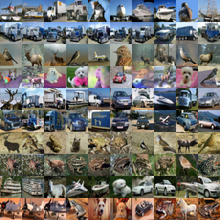Randomly sampled KNN examples 2

Tiny ImageNet

In each row, the leftmost image is the original query, and the 9 images to the right are the nearest neighbors, using cosine similarity. Results using Euclidean distance are similar.

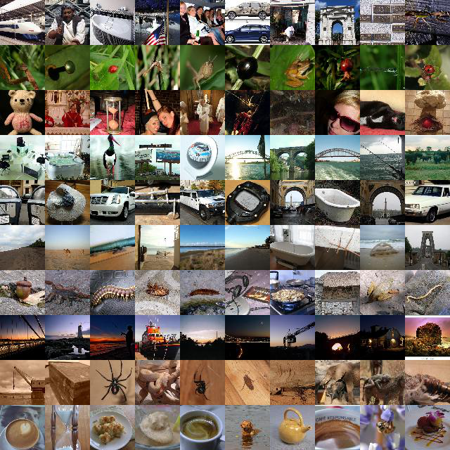Randomly sampled KNN examples 1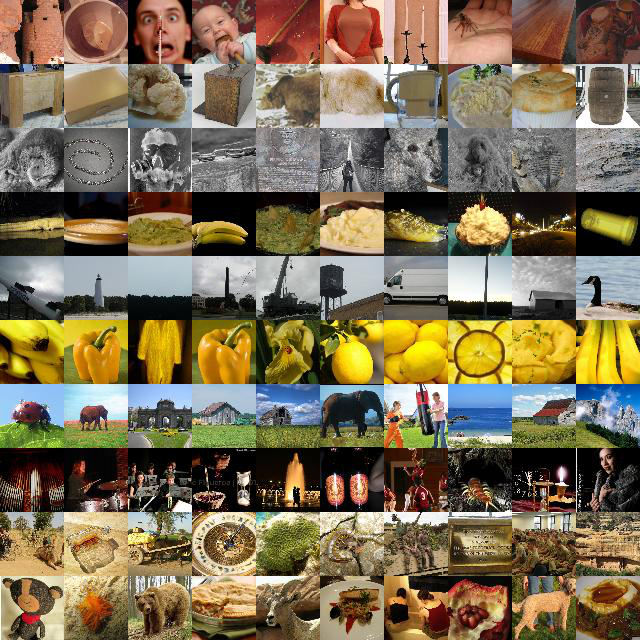Randomly sampled KNN examples 2

Global vs. Local

Introducing local mutual information turns out to be quite necessary — below is a comparison of KNN results using only global mutual information versus only local mutual information.

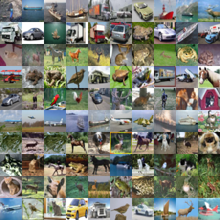Random KNN examples (global mutual information only)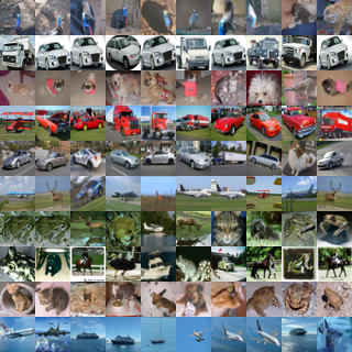Random KNN examples (local mutual information only)

Once Again, Journey's End

As a success story in unsupervised learning, this work generalizes and formalizes the concept of mutual information, which is common in NLP, and applies it to images. Of course, now that it's been abstracted this way, one could just as well bring it back to NLP, or apply it to other domains, since it's been formulated in a very general and applicable way.

I really like the overall style of the Deep INFOMAX paper: going from a general principle (mutual information maximization), to an estimation framework, to a concrete model, with clear reasoning and complete argumentation — it's my idea of what a good paper should look like (except for the use of adversarial training to handle the prior distribution, which I think is unnecessary). I look forward to seeing more papers written in this style.