WGAN-div: The Unsung Hero That Patched Up WGAN

WGAN-div：一个默默无闻的WGAN填坑者 苏剑林 · 2018-11-07 · Machine Learning GAN generative model metric

Today let's talk about the Wasserstein divergence, "W-divergence" for short. Note that this is a different beast from the Wasserstein distance (also known as the Wasserstein metric), which we'll call the "W-distance."

This post is based on the paper Wasserstein Divergence for GANs, which proposes a GAN training scheme called WGAN-div. This is a paper I greatly admire, yet it remains oddly obscure — I only stumbled upon it by chance while searching the literature. It doesn't seem to have caught on in either the Chinese or English-speaking communities, but I find it to be a remarkably elegant result.

If readers need a primer on WGAN, feel free to check out my earlier post The Art of Mutual Sparring: Getting Straight to WGAN-GP from Scratch.

WGAN

We know that the original GAN (SGAN) can suffer from vanishing gradients, and it was to address this that WGAN was born.

The W-distance

WGAN introduces the W-distance from optimal transport theory to measure the distance between two distributions:

\begin{equation}W_c[\tilde{p}(x), q(x)] = \inf_{\gamma\in \Pi(\tilde{p}(x), q(x))} \mathbb{E}_{(x,y)\sim \gamma}[c(x,y)] \end{equation}

Here $\tilde{p}(x)$ is the distribution of real samples, $q(x)$ is the fake (generated) distribution, and $c(x,y)$ is the transport cost — the paper uses $c(x,y)=\Vert x-y\Vert$. The notation $\gamma\in \Pi(\tilde{p}(x), q(x))$ means: $\gamma$ ranges over all joint distributions on $x, y$ whose marginals are $\tilde{p}(x)$ and $q(y)$. Intuitively, $\gamma$ describes a transport plan, and $c(x,y)$ is the cost of that plan; $W_c[\tilde{p}(x), q(x)]$ says we should find the transport plan with the lowest cost, and use that cost as the measure of distance between the distributions. more

The Dual Problem

The W-distance is indeed a good measure, but it's clearly hard to compute directly. When $c(x,y)=\Vert x-y\Vert$, we can convert it into the following dual problem:

\begin{equation}W(\tilde{p}(x), q(x)) = \sup_{\Vert T\Vert_L\leq 1} \mathbb{E}_{x\sim \tilde{p}(x)}[T(x)] - \mathbb{E}_{x\sim q(x)}[T(x)]\label{eq:wgan-d}\end{equation}

Here $T(x)$ is a scalar function, and $\Vert T\Vert_L$ is the Lipschitz norm:

\begin{equation}\Vert T\Vert_L = \max_{x\neq y} \frac{|T(x)-T(y)|}{\Vert x - y\Vert}\end{equation}

In plain terms, $T(x)$ must satisfy:

\begin{equation}|T(x)-T(y)| \leq \Vert x - y\Vert\end{equation}

Generative Models

With this in hand, training a generative model can be cast as a min-max problem under the W-distance:

\begin{equation}\mathop{\text{argmin}}_{G}\mathop{\text{argmax}}_{T,\Vert T\Vert_L\leq 1} \mathbb{E}_{x\sim \tilde{p}(x)}[T(x)] - \mathbb{E}_{x\sim q(z)}[T(G(z))]\end{equation}

The first $\text{argmax}$ tries to obtain an approximate expression for the W-distance, while the second $\text{argmin}$ tries to minimize that W-distance.

However, $T$ can't be arbitrary — it must satisfy $\Vert T\Vert_L\leq 1$, known as the Lipschitz constraint (L-constraint). How do we enforce this constraint? So on the one hand, WGAN opened up a whole new school of thought for GANs and pushed the theory to a new level; on the other hand, it also dug a giant hole regarding the L-constraint, a hole that has since drawn no shortage of researchers to... (jump in?)

The L-Constraint

Currently there are three main approaches to imposing the L-constraint on a model.

Weight Clipping

This is the approach proposed in the original WGAN paper: after each gradient descent step on the discriminator, clip the absolute values of the discriminator's parameters so they don't exceed some fixed constant.

This is a very crude approach and is essentially no longer used today. The underlying idea is: the L-constraint essentially requires that the network's fluctuation not exceed that of a linear function, and activation functions typically already satisfy this condition, so we only need to worry about the network weights. The simplest solution is to directly restrict the range of the weights, so that things don't oscillate too violently.

Gradient Penalty

This idea is very direct: since $\Vert T\Vert_L\leq 1$ can be guaranteed by $\Vert \nabla T\Vert \leq 1$, why not just add the discriminator's gradient as a penalty term to the discriminator's loss?

\begin{equation}T=\mathop{\text{argmin}}_{T} -\mathbb{E}_{x\sim \tilde{p}(x)}[T(x)] + \mathbb{E}_{x\sim q(x)}[T(x)] + \lambda \mathbb{E}_{x\sim r(x)}\Big[\big(\Vert \nabla T\Vert - 1\big)^2\Big]\end{equation}

But the problem is that we need $\Vert T\Vert_L\leq 1$ to hold everywhere, so $r(x)$ would need to be a uniform distribution over the whole space, which is clearly infeasible. So the authors adopted a rather clever (and slightly sneaky) trick: penalize along random interpolations between real and fake samples, thereby ensuring the L-constraint holds in the transition region between real and fake samples.

This scheme is WGAN-GP. It's clearly more sophisticated than weight clipping, and it usually works quite well in practice. But it remains an empirical scheme, without a more complete theoretical foundation.

Spectral Normalization

Another way to enforce the L-constraint is spectral normalization (SN); you can refer to my earlier post The Lipschitz Constraint in Deep Learning: Generalization and Generative Models.

Fundamentally, spectral normalization and weight clipping belong to the same category of approach, except spectral normalization has more complete theory and gives a looser (less restrictive) bound. There's another difference too: weight clipping is an "after-the-fact" treatment — the parameters get clipped directly after each gradient descent step, and this kind of post-hoc processing can itself cause instability during optimization. Spectral normalization, by contrast, is a "before-the-fact" treatment — it normalizes the spectral norm of each layer's weights before doing any computation, so spectral normalization becomes part of the model itself, which is more principled.

Although spectral normalization is more sophisticated, it shares a problem with weight clipping: it restricts the discriminator to a small cluster of functions. That is, the $T$ obtained after applying spectral normalization is only a small subset of all functions satisfying the L-constraint. This is because spectral normalization effectively requires every layer of the network to satisfy the L-constraint, but this condition is too rigid — perhaps one layer could violate the L-constraint while a later layer satisfies an even stronger version of it, such that the two cancel out and the network as a whole still satisfies the L-constraint overall. Spectral normalization simply can't accommodate this kind of situation.

WGAN-div

Against this backdrop, Wasserstein Divergence for GANs introduces the W-divergence, claiming that we can now dispense with the L-constraint entirely while still retaining the good properties of the W-distance.

Reviewing the Paper

Sounds too good to be true? Let's see what the W-divergence actually is. Right off the bat, the authors review some classic GAN training schemes, and then casually toss out a reference — Partial Differential Equations and Monge-Kantorovich Mass Transfer — which provides a scheme (presented here in a different order than in the paper) that lets us directly train $T$, with the objective (written slightly differently from the original)

\begin{equation}T^* = \mathop{\text{argmax}}_{T} \mathbb{E}_{x\sim \tilde{p}(x)}[T(x)] - \mathbb{E}_{x\sim q(x)}[T(x)] - \frac{1}{2}\mathbb{E}_{x\sim r(x)}[\Vert \nabla T\Vert^2]\label{eq:wgan-div-d1}\end{equation}

Here $r(x)$ is a very loosely constrained distribution, which we'll discuss further below. The meaning of the whole loss is: as long as you train $T$ according to this formula, it will be the optimal solution for $T$ in equation $\eqref{eq:wgan-d}$. That is, we can then plug it into equation $\eqref{eq:wgan-d}$ to obtain the W-distance, and minimizing that gives us the generator.

\begin{equation}\mathop{\text{argmin}}_{G}\mathbb{E}_{x\sim \tilde{p}(x)}[T^*(x)] - \mathbb{E}_{x\sim q(z)}[T^*(G(z))]\label{eq:wgan-div-g1}\end{equation}

A Few Notes

First, why do I say the author "casually" tosses out a paper? Because, well, that's exactly what happens...

The author simply writes "According to [19]" and then states the result that follows. [19] turns out to be a 59-page paper on optimal transport and PDEs... After much flipping through it, I finally figured out that the cited results should be on pages 36 and 40 (though even having found them, I still couldn't quite make sense of them, so I gave up). No further references are given either — how awkward. And for some of the later lemmas, the author simply says "just go read the discussion in [19]"...

The reader's next, more natural question is: how does this differ from the gradient penalty scheme? Isn't slapping a negative sign on it to turn it into a minimization pretty much the same thing? Maybe there's not much difference in practice, but theoretically the gap is enormous, because the gradient penalty of WGAN-GP is only an empirical scheme, whereas equation $\eqref{eq:wgan-div-d1}$ comes with theoretical guarantees. We'll finish working through this below.

The W-Divergence

Equation $\eqref{eq:wgan-div-d1}$ is a theoretical result, but deep learning, whatever else it is, remains a discipline that blends theory and engineering. So the author generalizes and considers the following objective:

\begin{equation}W_{k,p}[\tilde{p}(x), q(x)] = \max_{T} \mathbb{E}_{x\sim \tilde{p}(x)}[T(x)] - \mathbb{E}_{x\sim q(x)}[T(x)] - k\mathbb{E}_{x\sim r(x)}[\Vert \nabla T\Vert^p]\label{eq:wdiv}\end{equation}

where $k > 0, p > 1$. Building on this, the author proves that $W_{k,p}$ has some very nice properties:

1. $W_{k,p}$ is a symmetric divergence. By "divergence" we mean: $\mathcal{D}[P,Q]\geq 0$ and $\mathcal{D}[P,Q]=0\Leftrightarrow P=Q$ — the difference from a "distance" is that it need not satisfy the triangle inequality; such objects are sometimes called "semi-metrics" or "semi-distances." That $W_{k,p}$ is a divergence is already quite remarkable, because most GANs are, in effect, just optimizing some divergence. Being a divergence means that when we minimize it, we are genuinely shrinking the distance between the two distributions.
2. The optimal solution of $W_{k,p}$ has a definite connection to the W-distance. Equation $\eqref{eq:wgan-div-d1}$ is a special case of $W_{1/2,2}$. This tells us that once we've maximized $W_{k,p}$ to obtain $T$, we can drop the gradient term and train the generator simply by minimizing $\eqref{eq:wgan-div-g1}$. This also shows that using $W_{k,p}$ as the objective has properties similar to the W-distance and won't suffer from vanishing gradients.
3. This is, in my opinion, the most amusing point: the author proves that
\begin{equation}\max_{T} \mathbb{E}_{x\sim \tilde{p}(x)}[T(x)] - \mathbb{E}_{x\sim q(x)}[T(x)] - k\mathbb{E}_{x\sim r(x)}[(\Vert \nabla T\Vert - n)^p]\end{equation}
is not always a divergence. When $n=1,p=2$, this is exactly the gradient penalty of WGAN-GP, and the author is saying, in effect, that it's not a divergence — clearly taking a swing at WGAN-GP, ha! Not being a divergence means that when training the discriminator, WGAN-GP doesn't always actually widen the distance between the two distributions (the discriminator is slacking off instead of properly honing its discrimination skills), which means the gradient passed back to the generator during training can be inaccurate.

WGAN-div

Alright, after all that build-up, we can finally introduce WGAN-div, which is simply the WGAN training scheme based on $\eqref{eq:wdiv}$:

\begin{equation}\begin{aligned}T =& \mathop{\text{argmax}}_{T} \mathbb{E}_{x\sim \tilde{p}(x)}[T(x)] - \mathbb{E}_{x\sim q(x)}[T(x)] - k\mathbb{E}_{x\sim r(x)}[\Vert \nabla T\Vert^p]\\ G =& \mathop{\text{argmin}}_{G} \mathbb{E}_{x\sim \tilde{p}(x)}[T(x)] - \mathbb{E}_{x\sim q(z)}[T(G(z))]\end{aligned}\end{equation}

The former is meant to find the optimal $T$ in the W-distance via the W-divergence $W_{k,p}$, and the latter is meant to minimize the W-distance. So the W-divergence's role really is that of an unsung hero quietly patching up the W-distance — and combined with how little attention this paper itself has received, that impression only feels stronger to me.

Experiments

Choosing k and p

Through a batch of search experiments, the authors found that the best results (measured by FID) come from $k=2,p=6$. This further diverges from the WGAN-GP approach: the squared norm is not, in fact, the best choice.

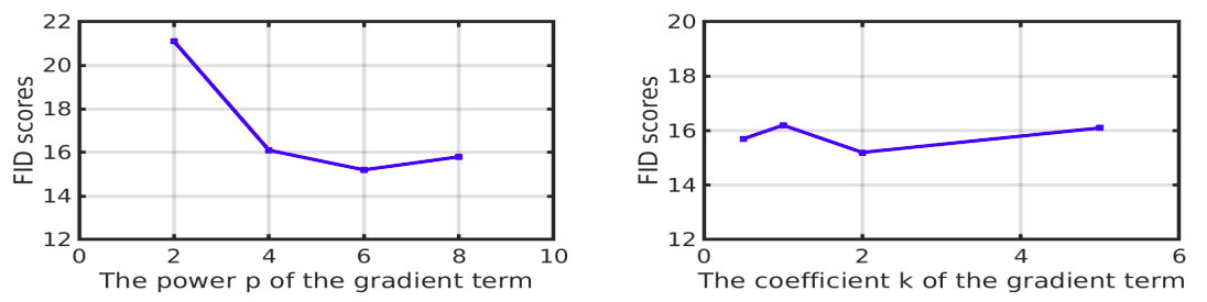
Effect of different k, p on FID (lower FID is better)

Choosing r(x) #

As mentioned earlier, the requirements on $r(x)$ in the W-divergence are extremely loose, and the paper runs a set of comparison experiments across common choices:

1. Random interpolation between real and fake samples;
2. Random interpolation among real samples, and separately among fake samples;
3. Mix real and fake samples together, then randomly pick two to interpolate;
4. Directly take a mixture of the original real and fake samples;
5. Directly take only the original fake samples;
6. Directly take only the original real samples.

The result: under WGAN-div, all of these choices perform about equally well (measured by FID), but under WGAN-GP, they differ quite a bit, and the best result under WGAN-GP is still worse than the worst result under WGAN-div. At this point WGAN-GP is thoroughly beaten...

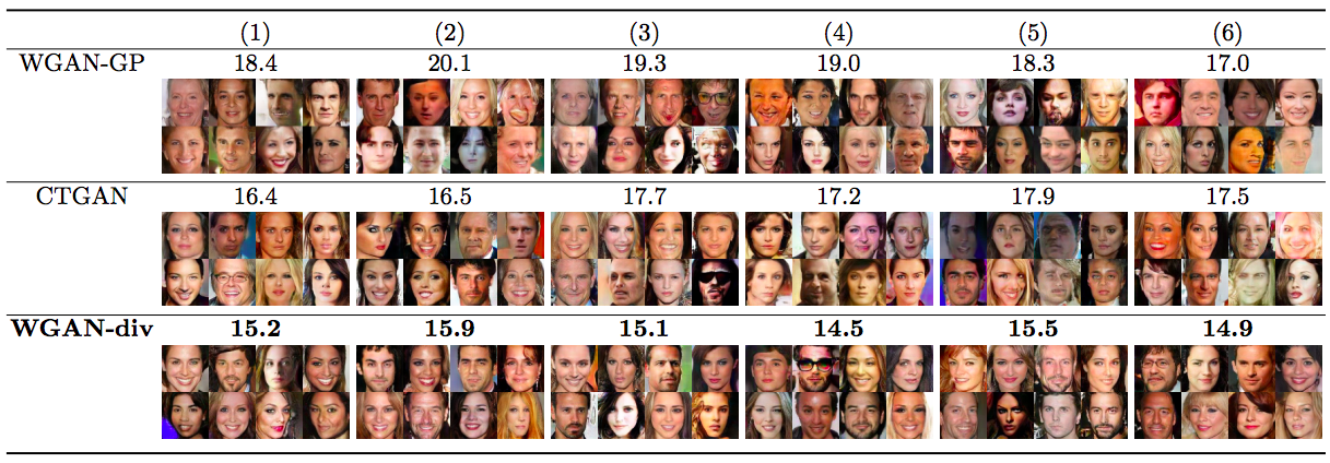
Different FID differences across models caused by different sampling schemes (lower FID is better)

The reason for this difference isn't hard to explain. WGAN-GP's gradient penalty is an empirical add-on, and "random interpolation between real and fake samples" is really just a compromise made necessary by the fact that it cannot sample the whole space. W-divergence and WGAN-div, by contrast, never impose any strict requirement on $r(x)$ from the outset, theoretically speaking. In fact, the original construction of the W-divergence (see the referenced paper for details) basically only requires that $r(x)$ be some distribution over a sample space matching $\tilde{p}(x)、q(x)$ — a very weak requirement. We generally choose it to be a distribution jointly derived from both $\tilde{p}(x)、q(x)$, since that tends to converge somewhat faster.

Reference Code

Naturally written in Keras — life is short, I use Keras.

https://github.com/bojone/gan/blob/master/keras/wgan_div_celeba.py

Random samples (from my own experiments):

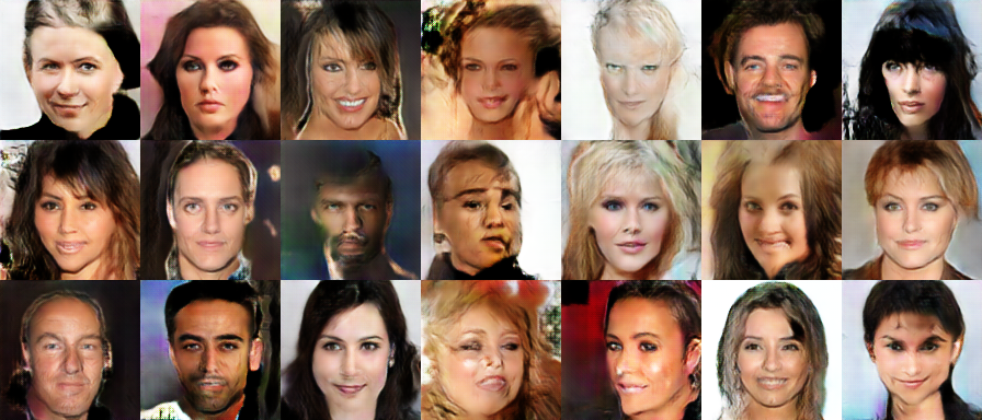
Some samples from WGAN-div (2w iterations)

And of course, the original paper's experimental results also show WGAN-div performing very well:

Comparison of WGAN-div against different models on different datasets (metric: FID, lower is better)

Closing Thoughts

I'm not sure how the field at large views this WGAN-div paper — perhaps people feel it isn't all that different from WGAN-GP and so there's nothing much to see here. But I have great admiration for the researchers who derive results like this from theory and use them to improve on the original — even if, along the way, they casually toss out a citation and say "figure it out yourself," the result of combining theory and practice this way still has genuine beauty to it.

I used to have some reservations about WGAN-GP — I always found it a bit ugly and was reluctant to use it. But now that WGAN-div has come along, it has replaced WGAN-GP in my heart, and it's no longer ugly at all.